In Part 1, we have studied how accounts of 3 individuals evolve in time, without considering any exchanges at all. But a currency without exchanges is a dead one.
You can download the spreadsheet for this part here.
Note on exchanges
Note that “not considering exchanges” doesn’t necessarily mean that the individuals don’t exchange at all, it only means that they have zero-sum exchanges. For instance, let’s consider that we have this situation every day:
I1 – Baker
I2 – Butcher
I3 – Grocer
Bread and cake
+50 UD
-50 UD
Steak and sausage
+50 UD
-50 UD
Veggies and fruit
-50 UD
+50 UD
Balance
0
0
0
They all exchange but numerically it looks exactly as if they didn’t exchange at all. Besides, we can note that those exchanges are very big compared to monetary creation: the GDP of this population is 300 UD per day! Yet everything looks as if they weren’t exchanging at all when considering the totals.
We see here the importance of considering economic flux and monetary creation separately.
(b) Simulate exchanges between I1 and I3
In this part, we will begin to examine what happens when the individuals perform non balanced monetary exchanges.
Some unbalanced exchanges in the absolute scale
So let’s consider that our 3 individuals perform mostly balanced exchanges in their lives, but that I1 and I3 do some unbalanced exchanges from time to time. Following is the relevant years when they exchange extra stuff along with the balance of their accounts at these years after the exchange:
Year
I1 account
I2 account
I3 account
I1 exchange
I3 exchange
12
128
88
128
50
-50
21
535
245
35
250
-250
31
67
677
1367
-900
900
49
276
3886
7576
-3000
3000
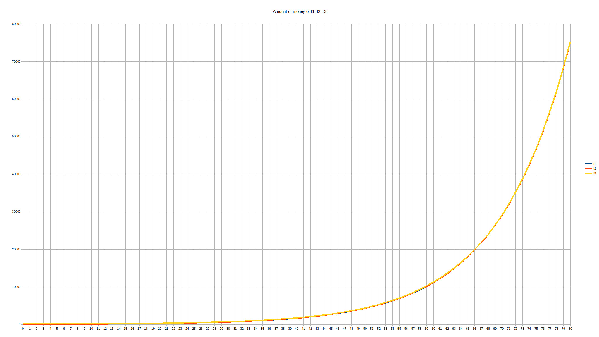
Unfortunately, the absolute scale doesn’t allow us to really see anything because of the exponential growth. Therefore we can switch to a logarithmic scale which allows to “flatten” things a little:
All accounts always converge toward the same value and that most exchanges are “forgotten” after a few decades, even the biggest ones.
In the relative scale
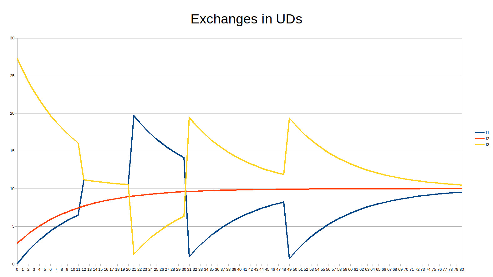
Now let’s switch to the relative scale and compute the same table of the exchanges expressed in UDs instead of absolute units:
Year
I1 account
I2 account
I3 account
I1 exchange
I3 exchange
12
11.2
7.7
11.2
4.3
-4.3
21
19.7
9.0
1.3
9.2
-9.2
31
1.0
9.6
19.4
-12.8
12.8
49
0.7
9.9
19.4
-7.7
7.7
At first sight, all accounts are roughly revolving around a mean value of 10 and thus the exchanges are expressed in values that don’t grow over time, unlike in the absolute scale. Let’s have a look at the chart of the exchanges:
It is interesting to note that you can even spend almost the average of all accounts (here 10) twice in a lifetime and still end your life with a full account. Even if you “rob” someone of their money twice in your life, you also end up with an account that is not significantly fuller than other accounts.
Daily unbalanced exchanges
Does this mean that one cannot get richer in a Libre currency, whatever you do? That is not entirely true. For instance, suppose that I1 is a very lazy person, or a person who produces Ğvalues which are not recognized by his peers during his lifetime as “values” thus not very well monetized, let’s call him Vincent (Van Gogh). In the meantime, I2 is a “regular” citizen who exchanges in a balanced way, let’s call him (Average) Joe. Finally, I3 is an extremely focused person whose goal in life is to produce values that are recognized by his peers, let’s call him Bill (Gates).
Let’s assume that, through his dedicated and intensive work, Bill manages to “catch” at time t 90% of a UD(t-1) per day from Vincent and 10% of a UD(t-1) per day from Joe. We don’t actually know what you can buy with a UD and these are only totals – maybe Vincent gives 50 UDs to Bill and gets back 49.1 UDs. One thing we know for sure is that Vincent cannot spend more than a UD daily on the long run – he would run out of money! So here we go, every day, we have:
Vincent
Joe
Bill
-0.9 UD
-0.1 UD
+1 UD
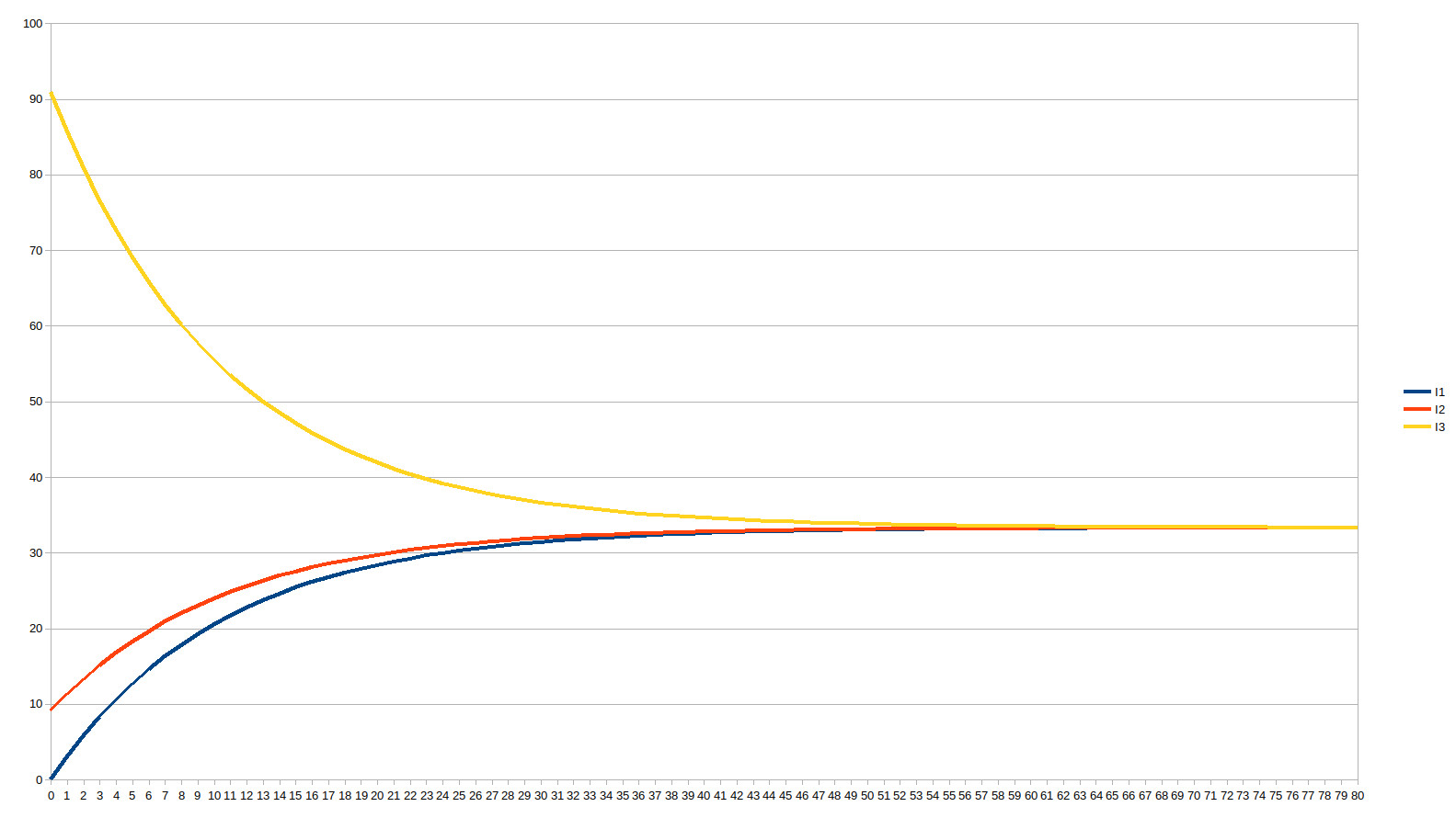
The corresponding chart in the relative scale looks like this:
It is now obvious that Bill, who takes from his father not only the monetary heritage but also the trading drive, has an account that tends toward 67 UDs, while Vincent, who not only didn’t have anything at birth but who also chose to produce not strongly monetized values, has an account that tends toward 3.3 UDs. Consequently, we have a whooping ratio of 30 between Vincent and Bill’s accounts.
Who said you can’t get rich in Libre money?
Well, you can get “richer than the others” but the main difference with other types of money is that you can’t get “insanely richer” than the others.
Let’s change the story
I have told on purpose a story where things seems quite “fair”. However, if you change the story, you may get something that could be definitely considered abnormal with exactly the same numerical values.
Alternatively, imagine that Vincent is not a painter, he’s actually a very hard working fellow in a factory owned by Bill. Vincent’s salary is ridiculous compared to the profits Bill gets from selling the objects made by his factory and from Vincent’s hard work. Besides, Bill is also the owner of the apartment where Vincent lives, so Vincent must pay him a rent. The story might end up like this: Bill is an extremely lazy guy who owns many things he inherited from his parents and live off of them, while Vincent is an extremely hard worker who kills himself trying to earn his life through 10+ working hours a days in a factory, but because he’s paid very little and has to pay for his rent, he ends up giving away 90% of his UD every day to Bill.
Obviously, the numbers are exactly the same, but the situation is totally different. Definitely, a Libre money system cannot fix all of society’s problems. However, because with Libre money we know how money is created and where it goes and the reasons why it goes there, then many schemes will be exposed while they remain hidden in the system’s complexity today. Because of that complexity and obscurity, we can always end up blaming the wrong people and the wrong things for the wrong reasons.
Finally, why would Vincent go enslave himself in a factory 10+ hours a day if he can actually live exactly the same life when painting at home? As he knows he has his daily UD, it will get harder to enslave him.
Welcome to the second part of my Galileo Module started there.
Please note that this post is a little technical. If you are not technically inclined, you could easily skip it.
Technical considerations on the precision of numbers
You can download the spreadsheet for this part here.
The world continuum
The world appears to be a continuous environment. Indeed, movements are smooth and don’t look like old animations like this one from an Iranian vase which is 4000 years old:
Similarly, light, sound, all seem to have a totally continuous space. Nobody knows for sure if everything is indeed continuous or if the “building blocks” are so small in both time and space that we cannot get to the level of precision needed to see them.
The discrete nature of computers
In the computer world, however, nothing is continuous. In time, everything depends on the “clock” of the microprocessor which can be thought as “beeps” at regular intervals. Similarly, in space, everything is coded as bits, pixels, etc. Nothing is continuous in the computer world, everything is “discrete”.
Computers use “bits” to store numbers. The less bits are used to store a number, the lower the precision of that number and/or the shorter range you can represent. With 8 bits, you can represent integers from 0 to 255, while with 16 bits, the range goes from 0 to 65535. But you could also choose to represent decimal numbers using 3 decimal digits from 0 to 65.535 with the same 16 bits. So the more decimal digits are used and the bigger the range we want to cover, the more bits are needed, which means more storage is used as well as we store the full history of all financial transactions.
We can make the parallel with the 3D industry. Depending on the precision of your “mesh”, 3D objects look smooth or horribly rough:
But if it is so, why don’t we use always smooth visuals? Because the first image is computed is mere milliseconds while the last one takes 10 minutes to build as well as much more memory. So there is a trade-off between time/space spent for calculations and how smooth we want things to appear.
In the music editing industry, the same kind of dilemma applies. All music is encoded in numbers that are stored in bits. If the data to be stored exceeds the capacity of the bits because the music’s volume was too high during the recording for instance, we experience what is called “clipping” which sounds pretty horrible and looks like this:
Consequences on UDs stored digitally
In a blockchain, all transactions are stored in a computer system. However, storage space costs energy, resources and money, it is important to minimize storage space. As transactions use a lot of numbers, it is worth investigating how much space we should use to store a number.
Using Integers
Let’s imagine that we wish to simply use integers to avoid storage costs. If we start with small numbers, we will have some “clipping” effects where we have to round numbers. The first problem we may face is that by rounding too much, we may not even be able to compute a UD that is greater than 0, for instance 3 × 0.1 = 0.3 which is rounded to 0:
Year
I1
I2
I3
N
Total
Total/N
UD
0
1
1
1
3
3
1
0
1
1
1
1
3
3
1
0
2
1
1
1
3
3
1
0
Okay, let’s use some higher numbers:
Year
I1
I2
I3
N
Total
Total/N
UD
0
1
5
9
3
15
5
1
1
2
6
10
3
18
6
1
2
3
7
11
3
21
7
1
3
4
8
12
3
24
8
1
4
5
9
13
3
27
9
1
5
6
10
14
3
30
10
1
6
7
11
15
3
33
11
1
7
8
12
16
3
36
12
1
8
9
13
17
3
39
13
1
9
10
14
18
3
42
14
1
10
11
15
19
3
45
15
2
We observe that for many years, the UD doesn’t change and remains at 1. The corresponding chart shows that the money mass doesn’t grow smoothly, its acceleration jumps when we switch from one integer to the next:
But it actually gets much worse than this. When we look at the relative scale, everything is expressed using the UD itself, which is rounded, so the curve is taking a very ugly form every time we switch from one UD to the next:
Decimals
Undoubtedly, using integers may be quite a bad idea. But it is mostly a bad idea because nobody wants to pay their bread 5.000 units of something. So let’s go on and use decimal numbers.
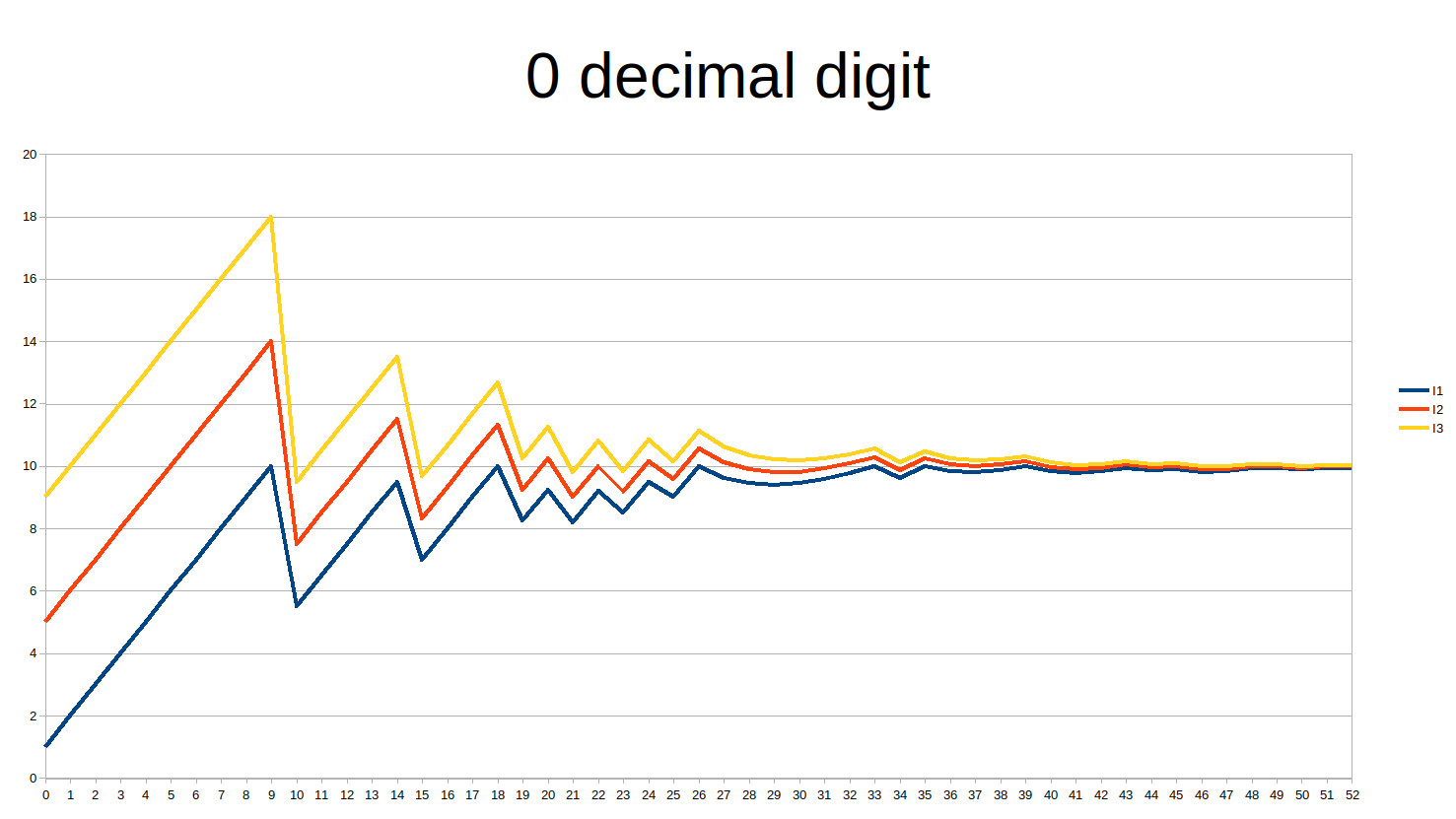
Let’s at least store a decimal digit:
It is better, but still not so great. Let’s try one more digit:
This is definitely better and quite acceptable.
Number of decimal digits
It is thus advisable to use floating point numbers with sufficient digits to compute the UD otherwise we may experience some “clipping effects” such as these. This effect diminishes as we advance towards greater numbers, but then the question of the possible range for our integers arises. If we have selected 16 bits to store integer values, the bad news is that, even if starting with very small values as above and with a population of only 3 individuals, the total money mass reaches 67.410 after 86 years, which will make it impossible to continue storing transactions at that time. Of course, a currency for only 3 people is pretty useless. We should consider for instance 3000 people instead which is a more likely and yet still timid scenario. Even then, we reach the same threshold after only 1 year and a month, and the more participants the quicker the limit is reached.
Moving the floating point
At some point, it is necessary to use a mechanism to move the floating point over time. Indeed, as time goes by, it becomes impossible to store exponentially growing values. Of course, we could grow the number of storage bits over time as well, which would be a rather bad idea! Instead, it is much more simple to move the decimal point which changes the base for counting in steps of 10x. We only need to store the current “base” to know in which base a specific number is expressed into.
Distributing the UD over time
So far, we have considered that the UD is created every year. But it is actually best to create is as often as possible, to smoothen the inequalities over time. If we distribute the UD every year on Jan 1st, it is clear that if someone enters the economic zone on Dec 31st, he has an advantage compared to someone who enters on Jan 2nd.
Theoretically, the UD would be created (or distributed) over time continuously at every millisecond, actually every nanosecond or femtosecond. Unfortunately, that is practically impossible as computers are machines that don’t operate continuously and require more energy to perform more calculations. We need to find a compromise between computer calculations vs generated inequalities. It could be created every hour, every day or even every week, whatever seems “acceptable” to the community using the currency.
This has some effects on the currency itself as every UD generation causes the number of monetary units to grow which causes a gap in the value of each unit (more units mean less value for one unit).
Updating the UD over time
Another reason for the clipping may also be that the UD will not be revised every microsecond, and not even every time the UD is distributed, as it is a costly operation. Currently in the Ğ1 currency it is only revised every 6 months while it is distributed every day.
Firstly, if there aren’t enough significant digits, then we might have a clipping effect every 6 months or more due to the revision of the UD, which is quite bad. Then, every time the UD is revised, it causes a “jump” in the relative scale of prices.
Let’s have a look at what happens if we revise the UD every 2 years instead of 6 months over a period of 40 years:
Have you noticed how the sawtooth effect is felt much more by the ones who own more money than the ones who own less? By the way, they don’t exactly experience minor changes on their accounts: the values suddenly drop by almost one third (exactly 28% in this case). This means that if people were to adjust prices, salaries and everything on the new DU, all prices would drop by 28% which is not acceptable for something that has only a purely technical cause that can be fixed.
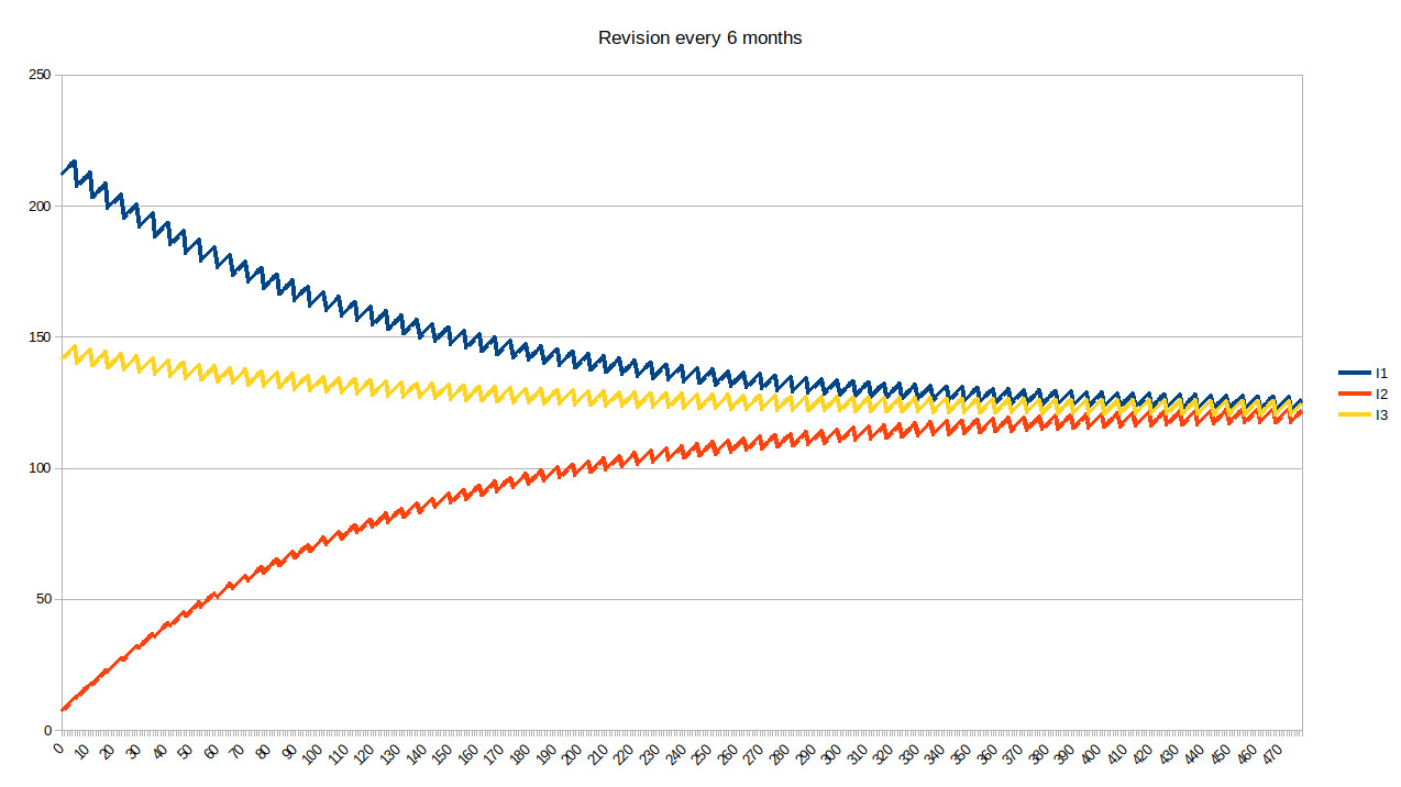
To fix this further, we can revise the UD every 6 months:
Obviously, the sawtooth effect is still there, but on a much limited scale (4%) which seems proportionally more acceptable. However, we could probably consider revising the UD more frequently to avoid such a sawtooth effect.
There is a lot of material available in French on the original Galileo Module, which I already translated into English. But because I believe it is important to spread the information to other places than French-speaking communities, I am releasing my own version of the Galileo Module in English. This version will also explain to the reader the basics of the Relative Theory of Money so that no prerequisite is needed to read this blog article. This first part addresses the first part of the Galileo Module about changing frames of reference in a libre currency.
What is a libre currency?
A libre currency as defined by M. Laborde in his Relative Theory of Money (which I will shorten to “RTM”) is a currency in which all individuals in an economic zone create money equally and at regular intervals. The amount of money created by all individuals is always a fraction of the existing money mass and every single individual at a given time creates exactly the same amount of money as the others. Thus, money is no more created by central entities, or banks, but rather by every living human, in full symmetry with his peers at a given time but also across generations. This is perfectly possible today thanks to blockchain technology. It is no coincidence in my opinion that the RTM was published in 2010, after the 2000 and 2008 crises but first and foremost shortly after the invention of the concept of blockchain in 2008.
(a) Changing Frames of Reference in Space
The spreadsheet for this part can be downloaded here.
Libre currency
We need to build a spreadsheet for the amount of libre money created by 3 individuals, I1, I2, and I3.
As explained above, libre currency functions as follows: regularly, every individual in the economic zone creates a share of money. This share of money is called a “Universal Dividend”. So at every interval, we need to calculate the total amount of money in circulation and multiply it by a celerity factor called c which is the percentage of the Universal Dividend. The result must then be divided it by the number of participants to get the Universal Dividend per person.
Note that the interval can be chosen randomly, but the shorter the better. In the current libre currency Ğ1 it is every day, but in this publication, we’ll stick to every year otherwise the spreadsheets could be quite huge!
The Absolute Reference Frame (counting monetary units)
Here is the beginning with 3 individuals I1, I2, and I3 who start in life with very different values in their accounts:
Year
I1
I2
I3
N
Total
Total/N
UD
c
0
0
10
100
3
110
36.67
3.67
0.1
N is the number of individuals
Total is the total amount of money available also called Money Mass, here it is simply the sum of the money of I1, I2, and I3
Total/N is the average amount of money available per individual
UD is the Universal Dividend per individual, which is Total / N × c
c is the celerity of the monetary creation, the percentage at which new money is created, here it is 10%=0.1. This means that the money mass will grow by 10% every year. Note that c cannot be chosen completely at random since it depends on the life expectancy of the population. 10% is an acceptable value for a population whose life expectancy is roughly between 35 and 80 years. For a population with an average 80 years life expectancy, the RTM predicts that values for c should be chosen between 6 and 10%.
At year 1, every single individual will create exactly one UD:
Year
I1
I2
I3
N
Total
Total/N
UD
c
0
0
10
100
3
110
36.67
3.67
0.1
1
3.67
13.67
103.67
3
121
40.33
4.03
We note right away that I1 has gone from 0 to 3+ units, while I2 sees a 30% increase of his money and I3 sees only a 3% increase in his money. The money mass is also growing which means that the UD for the next year is growing as well.
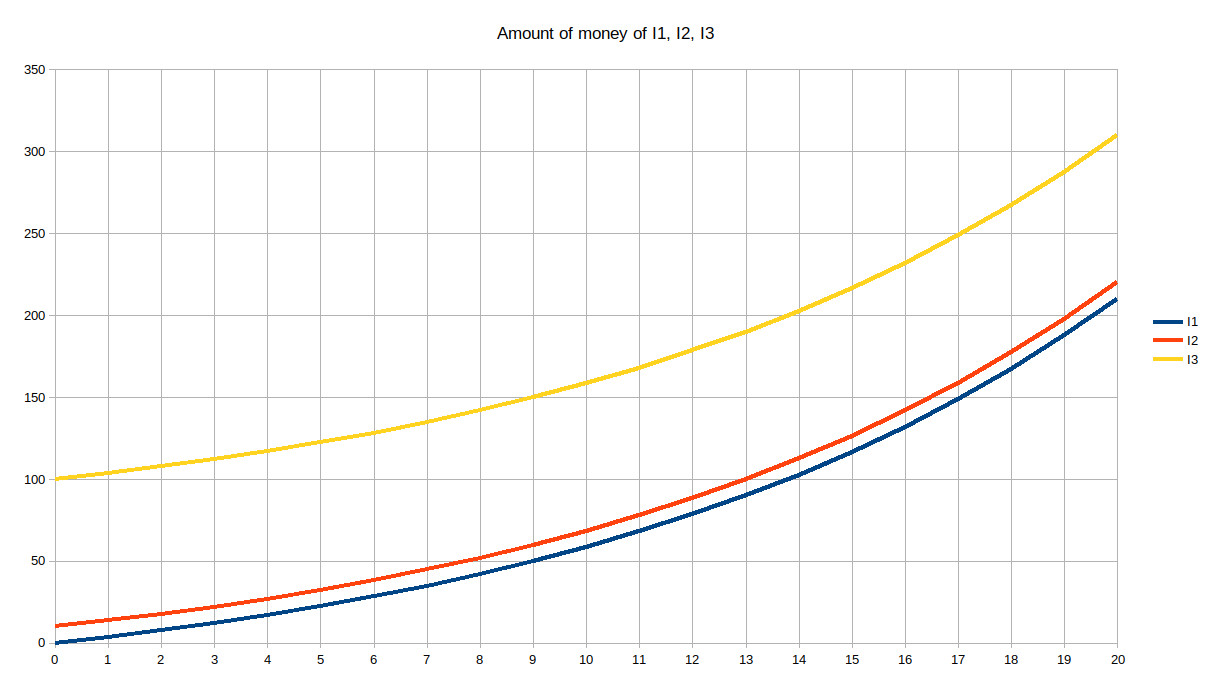
Because we are not computers I will stop showing the spreadsheet and show graphs instead which are much easier to read. Here is the graph of the amount of money over the first 20 years:
Unsurprisingly, this is an exponential curve. We can see that, over time, I1 who was the poorest, as well as I2 who was relatively poor compared to I3, are “catching up” with the richest – who still remains the richest. Now let’s extend this to 40 years, which is currently a half-life of a Westerner:
This time, it gets more difficult to see the difference between I1 and I2, and they are definitely catching up with I3. Let’s extend that to a full 80 years of life:
This time, the three curves are impossible to distinguish.
At first sight, this graph can be quite scary when we speak about money, especially about the total money mass. This reminds us of the Zimbabwe Dollar where an exponentially growing money mass is accompanied by exponential inflation, which is never a good thing when a state starts printing money like a crazy gambler:
The Relative Reference Frame (counting in proportion of the money mass)
Instead of counting monetary units, let’s change the frame of reference and use the percentage of the money mass as a reference.
Let’s go back to the first year of our 3 individuals and count how many percents of the existing money they possess:
Year
I1
I2
I3
Absolute
0
0
10
100
Percentage
0 %
9.09 %
90.9 %
I1 has 0%, I2 has 9% and I3 has 91% of the total monetary units.
We have seen that in year 1 the amount of money they have has changed quite a bit:
Year
I1
I2
I3
Absolute
1
3.67
13.67
103.67
Percentage
3.03 %
11.29 %
85.67 %
Now instead of representing the charts with the monetary units, let’s draw the chart for the percentage of money they own over time and during 80 years:
It is now very clear that I1 and I2 are getting a higher percentage of the money over time, at the expense of I3. All accounts are mathematically drawn towards the mean of all accounts.
We can already note that they approximately reach the mean after 40 years. This is because we have chosen the celerity to be 10%. Let’s see what happens when we choose 6% instead of 10%, as those are the bounds specified by the RTM for a life expectancy of 80 years:
This time, the mean is roughly reached only after 80 years, which is totally in sync with the predictions of the RTM: the highest recommended values of c cause accounts to converge within a half-life, while lower values of c cause accounts to converge within a full life.
We will now stick with the value of c = 10% in the rest of the article.
Both the graph in relative value and absolute value can be translated into references where the sum of all money is 0 at all times. In other words, at every moment, we check the difference between every account with the average total money per individual instead of the actual amount.
In this reference frame, the quantitative graph is quite surprising as it basically doesn’t move at all. Indeed, the absolute monetary difference between the individuals doesn’t change. It is proportionally very different when you consider the total money mass, but in absolute values, it never varies since we consider that our individuals give exactly as much as they receive (either because they don’t make exchanges at all, either because their exchanges are perfectly balanced):
On the other hand, the relative frame does show the shrinking differences between the three since it takes into account the percentage of money that each of them possesses:
Note that in this frame of reference, we have suddenly lost all thought of “hyperinflation” that could have worried us in the absolute frame of reference. After all, this is a very stable way of creating money!
Taxation
Now that we’ve studied what happens with a libre currency, let’s check what happens when we apply a fully proportional tax, eg. we take a fixed rate of tax on the accounts, calculated that way for an account R(t):
tax(t) = c × (R(t) + 1) / (1 + c)
The total collected tax is then redistributed equally among every single individual.
Let’s calculate the tax for the first year:
Year
I1
I2
I3
Total
T1
T2
T3
Total Tax
c
0
0
10
100
110
0.09
1
9.18
10.27
0.1
We can right away note that the tax on the rich is higher than the tax on the poor, which is normal since it is proportional. But we also note that there is an anomaly during the first year because the poorest has 0 and cannot be taxed. So we’ll adjust this special case to be 0 (is that fair – should he pay a tax to cover for this later?…). Now let’s see how it evolves over the next few years:
Year
I1
I2
I3
Total
T1
T2
T3
Total Tax
c
0
0
10
100
110
0
1
9.18
10.18
0.1
1
3.39
12.39
94.21
110
0.40
1.22
8.66
10.27
2
6.42
14.60
88.98
110
0.67
1.42
8.18
10.27
3
9.17
16.61
84.22
110
0.92
1.60
7.75
10.27
We see that we take the same amount of taxes every year (10.27) except the first year because of the anomaly of I1. Globally, the trend seems to be the same as in libre money: all accounts seem to tend toward one another. Here is the chart when counting monetary units:
As predicted, the accounts all converge towards the average. But note that this is the graph in absolute values now, whereas in libre money the quantity of money was growing exponentially. Now let’s have a look at the graph in relative values:
Unsurprisingly, it does look the same, the only change being the scale.
So the big surprise (or not!) here is that libre currency is equivalent to a certain form of tax redistribution. The pleasant surprise with tax redistribution is that we don’t need to “burden” ourselves with the relative reference frame since the quantitative reference frame with tax redistribution is already behaving the same way as the libre currency.
Let’s proceed and collect taxes for our perfect redistribution system and put the RTM in the trash can! (humor – read on!)
Thoughts on taxation systems
Let’s have a look at tax collecting systems and their efficiency in the history of mankind.
If you dig just a little, you’ll find that tax evasion today is absolutely everywhere. It is said to leak more than 1,500 billion (yes, 1,500,000,000…) dollars every year in Europe alone. Besides, there is “illegal” tax evasion, but there is also “legal” tax avoidance which, thanks to the very lenient tax laws in many countries, allow the richest to avoid paying much taxes. The funniest part is that the French government is definitely not looking at big tax evaders, but looking instead at petty and insignificant tax evaders. They are really not seeing the elephant in the room!
This is actually not new. Tax evasion has been around for a while, actually at least since lateAntiquity (2 different links).
In Ancient Greece, they actually found an original way of fighting tax evasion. Should we, too, incentivize our richest citizens to pay taxes in order to be revered and adored as benevolent philanthropists? Well, they already found the trick around that so it seems to be quite useless nowadays.
Let’s ask a simple question: why has tax evasion been always so popular? It is easy to explain: human nature is such that we hate to lose something, which is the case with taxes. On the other hand, creating money is always winning something so it is much easier to accept, even if you are actually losing in proportion!
Oh well. Let’s dig back the RTM from the trash can and read it one more time. 😀
Libre currency vs tax redistribution first and last round
The huge advantage of a libre currency compared to a tax-collecting system is that there is no avoiding taxes and their redistribution, which is then simply carried out mathematically through monetary creation. Ingenious!
Part 2 is a little bit technical so if you’re not into technicalities about computers, you should skip directly to Part 3.
“The Relative Theory of Money” is a book published in 2010 by a French engineer, Stéphane Laborde, who presents some very interesting thoughts and facts about money. He shows that, if we’re not careful enough, money creation can be the source of great inequalities. His book is a very good read for anyone, not only for those who wonder about money.
Within the book, many interesting questions are asked and answered. One of them is the “relativity of values”. To further study what is already analyzed in the book, the author offers a few “modules” in the form of exercises that can be done by anyone who wants to analyze further. Here is the translation in English of the first of these modules, the Galileo Module, the original (in French) can be found here: https://rml.creationmonetaire.info/modules/index.html
To be frank, at first sight it might look strange/gibberish if you’re not familiar with the RTM. I am publishing my own results of the module in English so that you can better understand what all this is about.
The Galileo Module
Theoretical data studies must be done from scratch.Economic data can be retrieved from various sources, or retrieved after verification of compliance from other contributors that have published their complete report of the module (which is the necessary condition to move to the next module).There are partial data known to date on the Duniter forum.
(a) Changing Frames of Reference in Space
create a spreadsheet representing a libre currency in the quantitative frame of reference with 3 individuals I1, I2, I3 over 80 years,
calculate the relative frame of reference,
create the two corresponding zero sum frames of reference,
create a separate sheet with the reverse relative / quantitative frames based on a tax which is redistributed using: individual tax(t) = c*(R(t)+1)/(1+c) collected and R(t+1) = R(t) + (collected tax(t) / 3) – individual tax(t)
perform a numerical analysis as well as a comparison of the graphs.
A Universal Dividend is equivalent to tax redistribution. Create a sheet and a graph to compare the two.
Avertissement : cet article traite de théorie de la musique, expliquée simplement aux musiciens ainsi qu’aux non musiciens, avec des mathématiques élémentaires (en utilisant des fractions simples). Le sujet est en fait assez méconnu, même des musiciens. À moins que vous ne sachiez ce que sont Werckmeister et Valotti, vous apprendrez quelque chose d’intéressant !
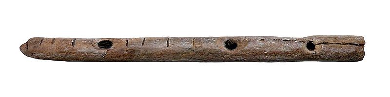
Depuis que la musique existe, les musiciens doivent accorder leurs instruments pour éviter de casser les oreilles de leur audience. Ce n’est pas seulement valable pour un orgue aux 20.000 tuyaux. L’un des instruments les plus simples, une flûte de bambou (ou d’os, quoi de plus romantique que de jouer son air préféré sur le tibia de votre chérie ? je plaisante…) avec des trous doit être construite avec minutie : un millimètre à côté, votre flûte sonnera faux.
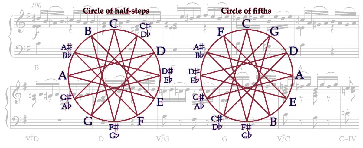
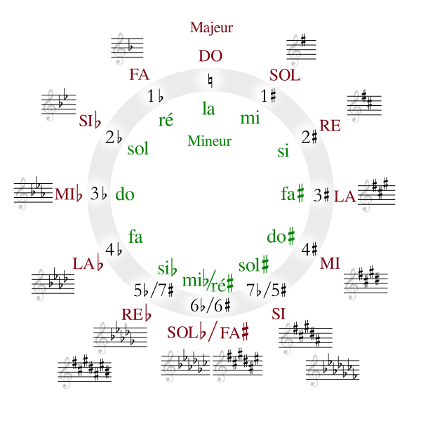
Il y a 2500 ans, Pythagore, avec les quelques instruments simples dont il disposait à son époque, se cassa la tête sur les mystères de l’accord des instruments et créa le désormais célèbre « cycle des quintes », exposant l’impossibilité d’accorder parfaitement un instrument, quel qu’il soit :
Pythagore comprit que la musique est essentiellement des mathématiques : les notes, les harmonies, la tonalité, les octaves, sont faites de fréquences et de la manière dont ces fréquences interagissent. Nos cerveaux et oreilles analysent les fréquences qui ont des relations mathématiques particulières entre elles comme harmonieuses, et les autres comme dissonantes. En réalité, le cerveau aime tout ce qui est mathématiquement « beau ». C’est la raison pour laquelle nous adorons les symétries telles que celle-ci :
Revenons à la musique. Lorsque deux notes sont jouées simultanément, elles forment un « intervalle », qui est la distance entre leurs fréquences sonores respectives. Un intervalle est agréable à l’oreille lorsque les fréquences des deux notes qui le composent sont mathématiquement liées par une fraction entière. Dès que les fréquences des deux notes s’éloignent d’une telle relation mathématique, l’intervalle sonne faux, il casse les oreilles. D’ailleurs, un intervalle qui s’éloigne de cette perfection mathématique se met à créer des interférences et à « battre », ce qui est très pratique pour accorder des intervalles avec précision sur un instrument de musique. L’oreille est un organe très délicat et très précis.
Laissons la théorie pendant un instant et faisons un peu de pratique ! J’ai enregistré une quinte (5 notes d’écart sur un clavier de piano), l’intervalle Do-Sol sur mon épinette. L’épinette est un petit clavecin qui n’a qu’une seule corde par note, ce qui rend les choses plus faciles à entendre. Pour commencer, écoutons une quinte parfaitement accordée. Elle sonne juste, et surtout le son est régulier, il diminue d’intensité progressivement et sans à-coups (il est préférable d’utiliser un casque) :
Visuellement, le son ouvert dans un logiciel permettant de voir la forme des sons est une courbe descendante sans grande particularité :
Maintenant, désaccordons très légèrement le sol. L’accord se met à « battre », comme le montre la vidéo suivante. N’hésitez pas à la réécouter en suivant l’indication visuelle, jusqu’à ce que vous entendiez ces vagues qui font « wow, wow, wow… » :
Et lorsqu’on regarde la forme du son, les battements sont déjà visibles :
Désaccordons encore un peu plus le sol. Les battements sont plus rapides. À noter que ce n’est pas un effet digital, l’épinette sonne réellement exactement comme ça :
Cette fois, la forme du son indique très clairement ces battements :
Et pourtant, la seule chose que nous ayons fait ici est de changer très légèrement le sol, le faisant dévier de moins de 1% de sa valeur parfaite !
Regardons maintenant les différents intervalles qui peuvent être formés.
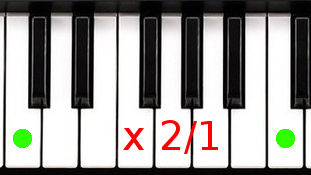
Prenons une fréquence et son double, on obtient une octave. Par exemple 440 Hz et 880 Hz.
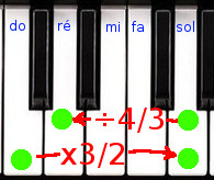
Prenons les 3/2 d’une fréquence, on obtient une quinte parfaite.
Les 4/3, une quarte.
Les 5/4, une tierce majeure.
Les 6/5, une tierce mineure.
Dès que deux notes ne suivent pas ces intervalles précis, leur combinaison sonne faux et l’intervalle commence à « battre ».
Pour l’instant, tout va bien. Avec ce qu’on vient de voir, on pourrait tout simplement dire qu’il ne nous suffit plus qu’à accorder notre instrument avec des intervalles parfaits, et le tour est joué !
Sauf qu’en réalité, c’est là qu’intervient le problème : il est mathématiquement impossible de découper une octave en douze notes (les demi-tons) de manière à obtenir des quintes parfaites, sans même parler de quartes ou tierces parfaites. Pourquoi donc ? Ne nous en tenons pas à cette affirmation péremptoire, démontrons-la.
Une octave parfaite sonne généralement très bien. C’est la combinaison d’une fréquence et de son double, le cerveau est pleinement satisfait de la perfection mathématique qui en résulte. D’ailleurs, lorsqu’elle est parfaitement accordée, il est même parfois difficile d’entendre deux notes distinctes tellement elles se marient impeccablement. Arrivez-vous à entendre deux notes distinctes de cette octave enregistrée sur mon épinette ?
Avec son cycle des quintes, Pythagore, qui avait décidément d’autres choses en tête que des triangles, montra que, si on voulait accorder un instrument avec des quintes parfaites, les octaves que l’on obtiendrait sonneraient comme cela :
Ouille ! Vous allez avoir besoin de vous gratter les oreilles après une telle horreur. Je vous invite à réécouter l’octave parfaite au-dessus pour rétablir un certain calme dans votre oreille et votre cerveau agacé par autant d’imperfection.
Pythagore utilisa de nombreuses quintes et octaves pour faire sa démonstration, mais nous pouvons nous contenter de 5 notes pour aboutir au même résultat.
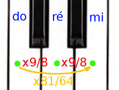
Calculons la différence entre un do et un ré de manière à avoir des notes parfaites. Do-sol est une quinte, c’est donc un intervalle 3/2 comme nous l’avons vu dans la table précédente. Cela veut dire que la fréquence du sol est 3/2 plus grande que la fréquence du do. D’autre part, ré-sol est une quarte, elle doit donc suivre un intervalle 4/3. Ce qui signifie que pour passer du sol au ré, nous devons diviser par 4/3.
sol = do × 3/2
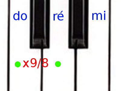
ré = sol ÷4/3 = sol × 3/4 = (do × 3/2) × 3/4 = do × 9/8
Ré est donc 9/8 de la fréquence de do si on veut avoir des intervalles parfaits. Excellent ! Ce ne sont là que des mathématiques simples, passant d’une note à l’autre à l’aide de fractions.
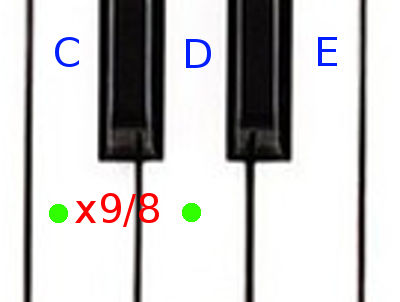
Calculons maintenant la différence entre do et mi. Facile. Do-ré est un ton, ré-mi est également un ton, il y a donc également 9/8 entre ré et mi.
Ce qui veut dire que, pour passer de do à mi, il suffit de multiplier par le carré de 9/8, soit 81/64. Et 81/64 ≈ 1,265.
Une petite seconde ! Do-mi est une tierce majeure. Nous avons vu dans la table plus haut que les tierces majeures parfaites suivent un intervalle de 5/4. Mais 5/4 est égal à 1,25, pas 1,265. Pas loin. Mais pas exactement identique. Voilà notre première déception : si on veut construire ré de manière à avoir des intervalles justes, alors notre tierce do-mi ne peut pas être parfaite. On peut déjà imaginer que ce qui est vrai pour cette tierce va être également valable pour bien d’autres intervalles.
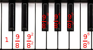
Par exemple, essayons de reconstruire une octave avec notre gamme composée de tons valant 9/8 chacun. Do-ré est 9/8, do-mi est 9²/8² (9/8 fois 9/8), do-fa# est 9³/8³, etc. :
Une octave composée de 6 tons est donc 9⁶/8⁶ ≈2,0273. Nous avons vu qu’une octave doit avoir un ratio d’exactement 2 pour être parfaite, pas 2,0273. Et voilà comment la perfection en musique disparaît sous nos yeux ou plus exactement nos oreilles. Et vous avez déjà entendu à quoi ressemble une octave à 2,0273 au lieu de 2, c’est tout simplement horrible ! Écoutons-la encore :
Il nous faut donc accepter un fait qui est dur à avaler : diviser une octave en douze notes ne va jamais nous permettre d’obtenir des quintes, quartes et tierces exactes. Des approximations très proches, mais jamais exactes. Quelle que soit la manière dont vous allez accorder votre instrument, il ne produira jamais d’harmonie parfaite. Quelle pensée agaçante pour un musicien ! Aussi parfaite que soit sa musique, elle sonnera toujours faux ! Et d’ailleurs, si l’on n’est pas extrêmement vigilant, certaines portions risquent même de casser sérieusement les oreilles.
Nous n’allons pas rentrer dans davantage de détails. L’essentiel est d’avoir compris que la perfection en musique est tout simplement inatteignable, et que pour produire 12 notes dans une octave européenne, il faut faire des compromis : si l’on veut que certains intervalles soient presque parfaits, il va nous falloir en « sacrifier » certains autres. Plus les uns sonneront à la perfection, plus les autres sonneront faux. Alors, certaines quintes ne seront pas exactement de 3/2, des quartes et tierces dévieront sensiblement de leur ratio parfait. En fait, tout va sonner un peu faux. Le but de l’accordeur et du compositeur est de minimiser les frictions dans l’oreille venant de ces imperfections. Pythagore a montré qu’on peut effectivement accorder la majeure partie d’un instrument de manière presque parfaite, mais qu’on obtient alors inévitablement un intervalle atroce qui sonne terriblement faux qu’on appelle typiquement « la quinte du loup », tellement cet intervalle sonne comme le hurlement d’un loup.
Depuis Pythagore, de très nombreux musiciens ont tenté de trouver une solution à ce problème, d’une manière ou d’une autre, découpant l’octave en 12 notes de manières toutes plus ingénieuses les unes que les autres. Ces différentes variations, ces différents découpages, sont appelés « tempéraments ». Cela peut évoquer aux amoureux de musique classique le titre de l’œuvre de J.S. Bach « Le clavier bien tempéré ». Au XVIIIème siècle, il existait de nombreux tempéraments, chacun avec ses avantages et inconvénients, la plupart n’autorisant pas de jouer dans certaines tonalités, comme le Werckmeister et le Valotti que j’ai cités en début d’article. L’œuvre de Bach « Le clavier bien tempéré » utilise de très nombreux intervalles pour montrer de manière pratique les applications du tempérament qu’il avait développé et qui permettait de jouer dans n’importe quelle tonalité sans problème et sans être gêné par une quinte du loup.
D’autre part, dans chaque tempérament, les musiciens réalisèrent que chaque tonalité avait sa propre « humeur », certaines tristes, d’autres joyeuses, d’autres encore inspirant l’angoisse, à cause des différents intervalles majoritairement utilisés dans chaque tonalité qui sonnent plus ou moins juste. Du coup, ces musiciens se mirent à choisir très précisément la tonalité et le tempérament de leurs compositions en fonction de l’atmosphère qu’ils voulaient leur donner.
Voici un exemple de classification par différents compositeurs comme Charpentier ou Rameau:
Do majeur : joyeux
Do mineur : triste, deuil, chagrins amoureux
Ré majeur : drôle, triomphant, victorieux
Ré mineur : calme, grave, tendre, dévot
Mi b majeur : pathétique, cruel, sévère, dévot
Mi b mineur : horrible, anxieux
…
Fa majeur : tempête, furieux
etc.
De nos jours, un tempérament particulier est devenu la référence pour presque tout le monde (excepté la musique baroque et renaissance, principalement) : le « tempérament égal ». Il fut inventé il y a plusieurs siècles et même décrit autour de 400 de notre ère par un mathématicien chinois, et bien que des méthodes existent depuis le XVIIIème siècle pour l’accorder à l’oreille, il ne peut être réellement atteint qu’à l’aide de la précision des instruments électroniques. Ce tempérament, plutôt que de faire des compromis et favoriser tel ou tel intervalle, rend chaque intervalle aussi bon/mauvais que les autres. Il consiste simplement en un découpage de l’octave en 12 parts parfaitement égales. Son acceptation n’a pas été facile et certains musiciens le critiquent encore aujourd’hui : il n’a pas de « couleur ». Que vous jouiez votre morceau en do ou en sol# n’a aucune importance, il sonnera toujours pareil, à une hauteur différente, mais avec les mêmes harmonies. Dans tous les autres tempéraments, comme on a pu le voir, chaque tonalité a sa propre « humeur ». Il est même parfois impossible de jouer dans certaines tonalités parce que cela sonne horriblement faux, comme si on jouait sur un de ces pianos désaccordés des bars des années 1900 aux États-Unis. En tempérament égal, rien ne sonne parfaitement juste mais rien ne sonne totalement faux non plus. Aucun intervalle n’est parfaitement juste à part les octaves. Notre oreille s’y est habituée avec le temps mais l’expérience d’écouter d’autres tempéraments peut parfois être une vraie révélation pour certains. Tout dépend de votre oreille, de vos attentes, de votre envie de découvrir autre chose, etc.
Nous allons nous arrêter là pour cette rapide introduction sur les tempéraments en musique. C’est un sujet qui a fait couler beaucoup d’encre et alimenté les conversations pendant des millénaires. Et c’est loin d’être terminé car des gens se penchent toujours sur le problème, tentant des nouvelles approches pour découper l’octave de différentes manières par des compromis différents, frustrés par la totale imperfection du tempérament égal. J’espère que cet article vous aura intrigué, vous aura fait approcher la musique sous un angle différent et montré ce problème pourtant simple qui agace les musiciens depuis que la musique existe.
Pour des exemples sur la manière dont différents tempéraments affectent la sonorité de la musique, vous pouvez vous rendre sur la page wikipedia (en anglais, mais il suffit de cliquer sur les boutons ► à droite, on entend clairement les intervalles qui sont vraiment faux, le premier exemple en “just intonation” est particulièrement horrible dans certains passages).
Foreword: this article is about music theory, explained to non-musicians and musicians alike, with very simple math (all you need is basic fractions). Unless you know Werckmeister and Valotti, you will definitely learn something cool from this article. 🙂
Musicians have always had to tune their instruments to avoid having their audience’s ears bleeding. This is not only true for an organ that has 20,000+ pipes. One of the simplest instruments, a flute made of a stick of bamboo (or a bone, can you think of anything more romantic than playing your favorite tune on your sweetheart’s tibia?… just kidding) with holes in it has to be constructed very carefully: move a hole by a single millimeter, your flute will sound out of tune.
2500 years ago, Pythagoras, with the limited instruments of the time, racked his brain on the problem of tuning and finally devised the “circle of fifths”, exposing the impossibility to tune any instrument perfectly:
Pythagoras understood that music is essentially mathematics: notes, harmonics, pitches are all about different frequencies and how these frequencies interact with each other. Our brains and ears recognize matching frequencies as harmonious and non matching frequencies as dissonant. In fact, the brain loves everything that is mathematically related. That is why we love symmetries such as these:
Back to music. When two notes are played together, they form an “interval”, which is the distance between their respective frequencies. Intervals sound great to the ear when the frequencies of the two notes composing the interval are mathematically related by integer fractions. If they are out of tune and too far from a perfect ratio, they start sounding bad. Besides, any listener will hear “beats” as soon as the interval is a little off, which makes it easier to tune perfect intervals with a very good precision, the ear is a very delicate and precise organ.
Let’s hear what it sounds like! I have recorded a simple fifth, C-G, on my spinet, an instrument that has only one string per note, which makes hearing things more simple. First, let’s listen to a fifth that has been perfectly tuned, it sounds regular, fading away slowly (for best results, use a headset):
Visually, the sound wave is a gradually decreasing sound:
Now when this fifth starts getting out of tune, it starts “beating”, follow the visual indication. If needed, play the video a couple of times until you clearly hear the beats:
The beats clearly show on the audio wave:
Finally, when the fifth is clearly out of tune, the beats get faster, note that this is not a digital sound effect, this is exactly how it sounds on my spinet:
And when looking at the sound wave, the beats are even more visible:
And the only thing I did was to change the G very slightly, actually less than 1% of its perfect value!
Now, let’s have a look at the different perfect intervals that can be formed.
Take a frequency and its double: you have an octave. For instance 440 Hz and 880 Hz.
Now take 3/2 of a frequency, you have a harmonious fifth.
Take the 4/3, you get a fourth.
5/4, a major third.
6/5, a minor third.
Remember, as soon as two notes don’t respect these perfect intervals, they start sounding “off” and their combination starts “beating”.
So far, so good, everything looks pretty simple, we just need to tune our instrument using perfect intervals, et voilà!
But here comes the problem: it is mathematically impossible to slice an octave into 12 notes (called semitones) that have perfect fifths, forget even about perfect fourth or thirds. This assertion might sound blunt. We need proof! Let’s dig into the problem.
An octave is generally very “round” to the ear. It’s the combination of a frequency and its double, the brain is very satisfied with that. In fact, when tuned correctly, it is even sometimes difficult to say that there are actually two notes there, they “blend” perfectly. Can you hear the two notes here making an octave:
With his circle of fifths, Pythagoras proved that, if you wanted to tune your instruments so that it would have perfect fifths, your octave would sound like this:
Ouch! Your ears could do with some little extra care now. You can listen to the perfect octave above to get away from this annoying sound ringing in your ear. While Pythagoras used many fifths and octaves to prove this, we can actually use just 5 notes to demonstrate it.
Let’s calculate how much we have between C and D if we want to maintain things perfect. C-G is a fifth, so it is a 3/2 interval, as we have seen in the table just above. This means that G is 3/2 of C. D-G is a fourth, so it is a 4/3 interval. Which means that to go from G down to D, we have to divide by 4/3:
G = C × 3/2
D = G ÷4/3 = G × 3/4 = (C × 3/2) × 3/4 = C × 9/8
So D is 9/8 of C when building it with perfect intervals. Great. This is just simple math, jumping from one note to the other using basic fractions.
Now, let’s see what we have between C and E. E must also be 9/8 of D, as it is a normal tone in the scale, no different than C-D.
So E must mathematically be 81/64 of C. And 81/64 ≈ 1.265. Wait a second. C-E is a major third. We have said earlier that perfect major thirds use a 5/4 interval. However, 5/4 = 1.25, not 1.265. Close. But not exact. That’s our first “uh-oh” problem: when we use perfect intervals to build the interval C-D, we can no longer create perfect intervals for the major third C-E, and you can guess that it will also be the case with other intervals.
For instance, let’s go on to the next octave using 9/8 as a step for a tone. C -> D is 9/8, C -> E is 9²/8² (9/8 times 9/8), C -> F# is 9³/8³, etc.:
So an octave constructed with 6 tones is actually 9⁶/8⁶ ≈2.0273. But we said an octave needs to have a ratio of 2 to sound perfect, not 2.0273. Oh well, here goes perfection in music! And you heard what 2.0273 instead of 2 sounds like before, it’s simply horrible! Let’s play it again:
At this point, we have to accept one fact that is hard to swallow: dividing an octave into 12 notes is never going to produce exact fifths, fourths or thirds. Very close approximations of them, but never exact. However you tune your notes, they will never sound perfect. Such an annoying thought for a musician! However perfect his music is, it will never sound right! And not only will it not sound perfect, some of it will sound pretty nasty if you’re not extra careful.
We will not go into much more detail. At this point, you came to realize that when cutting an octave into 12 notes to produce the standard European scale, you have to make trade-offs: if you want some intervals to sound close to prefect, some other intervals will have to be sacrificed. Some fifths will not be exact 3/2 intervals. Some thirds will be really off from their exact intervals. Mostly everything will be off, really, ever so slightly. The goal is to find a slicing that minimizes the roughness in the ear coming from all these intervals that are off. Pythagoras showed that you could tune most notes almost perfectly but that you would then have an inevitable rogue interval that would sound so terrible that it is called a “Wolf interval” since it howls like a wolf when you hear it!
Many musicians since Pythagoras have tried to address the problem in one way or another, designing “the best slicing” of their choice. These different variations in slicing the octave cake are called “temperaments”. If you know a little about classical music, this could remind you of the title of J.S. Bach’s “Well-Tempered Keyboard”. In the 18th century, there were many different temperaments, each suffering from various problems when playing in different keys, such as the Werckmeister and the Valotti cited in the prologue of this article. Bach’s work “The Well-Tempered Keyboard” uses many intervals in order to give a practical demonstration of his temperament in which you could play in various keys without problem and without hearing any wolf interval.
Besides, with a given temperament, musicians started to understand that every key had a different “mood”, some sad, some scary, some joyful, due to the different parts of the melody that sounded rounder or harsher than the others depending on which intervals they were using most. Therefore, they chose the keys of their compositions very carefully.
Here is an example of a classification from various composers such as Charpentier or Rameau:
C major: joyful
C minor: sad, mourning, love sorrow
D major: funny, triumphant, victory
D minor: calm, grave, tender, devotion
E flat major: pathetic, cruel, harsh, devotion
E flat minor: horrible, anxiety
..
F major: storm, furious
etc.
Nowadays, one temperament is used almost universally (except for baroque players, mostly): the “equal” temperament. It has actually been invented some centuries ago (in fact, a Chinese mathematician described it around 400 AD), but it can be tuned perfectly only with the precision of electronic devices (although there are methods to reach very good approximations of it, people began to use it in the 18th century). Rather than making compromises, the equal temperament makes every single interval as equally good/bad as the others. Basically, the octave is cut into 12 absolutely equal pieces. This is why some musicians criticize it and why it faced some resistance before being adopted: it has no “color”. Whether you play your tune in C or in G flat, it will sound exactly the same, at a different pitch, but with the same harmonics. In other temperaments, as we have seen, every key has its own “mood”. You may not even be able to play some keys in some temperaments because they will sound hideous, as if you were playing on one of those out of tune pianos in the pubs of the 1900s. But in equal temperament, nothing sounds exactly right at all, it is just never totally hideous either. In fact, in the equal temperament, no single interval is perfect, except for the octave.
This is it for a very short introduction to music theory of temperaments. Many books have been written on the subject, and it is still not over as people still come up with new ideas to get the best compromises out of a scale. I hope this has intrigued you and made you wonder a little more about this simple problem that has annoyed musicians for thousands of years.
For some examples of how a temperament can affect how you hear things, you can have a look at the Wikipedia page for musical tuning and listen to the samples in the “Systems for the twelve-note chromatic scale” section, the “just intonation” is particularly telling!
Deuxième vidéo d’une série sur la blockchain. Si vous avez entendu parler de cette technologie mais que vous vous posez des tas de questions, cette série est faite pour vous !
Après avoir donné un rapide historique et les divers usages de cette technologie dans la première vidéo, on s’attaque cette fois à ce que c’est un peu plus en détail sans pour autant virer dans la technique.
Visible aussi sur youtube : https://youtu.be/Zhvq0wE8F3Q
I’ve just unmounted my drives from my Synology box, replaced by a home-brewed server. I’ll write some other article about the reasons that made me switch. Just in case you wonder, the Synology box is running fine. That’s not the point.
I took the disks from the Synology box and plugged them into a host with simple Linux distrib (in my case, Ubuntu, but that shouldn’t matter).
Just type:
mount /dev/vg1000/lv /mnt
That’s it. You have the file system from your Synology box on your Linux machine. It may come handy in case your box crashed and you are waiting for a new one. In the meantime, you have access to your data.
In case you want to reuse the disks and dispose of them (WARNING: the following will destroy your data on those disks), here is how to do it.
vgremove vg1000
Now check the md volumes that are available and that you didn’t create yourself (just use ls /dev/md12*). Then stop those volumes (replace md12? with the volumes you want to stop if you have additional ones on your system that you obviously don’t want to stop – they won’t stop if they are mounted anyway):
mdadm -S /dev/md12?
Empty the beginning of the related disks, for each disk replace the … by your disk letter:
dd if=/dev/zero of=/dev/sd… bs=1M count=1024
And now you can play around with partitioning etc without being bothered again by vg1000 or mdadm.
Première vidéo d’une série sur la blockchain. Si vous avez entendu parler de cette technologie mais que vous vous posez des tas de questions, cette série est faite pour vous !
Visible aussi sur youtube : https://www.youtube.com/watch?v=6xOyBMkRcHQ
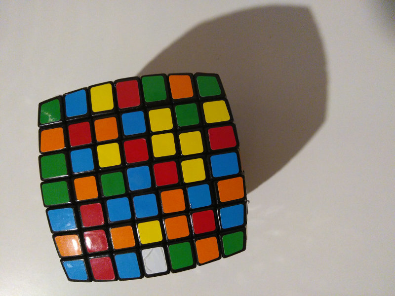
Two years ago, my wife offered me a very nice gift:
While that was a great gift and the kind of challenge that I would take on, I felt embarrassed as I even had no idea how to solve this:
Right.
And at the same time, I remembered how, as a child, I had swapped stickers on a 3×3 Rubik’s cube in the hope of solving it. Embarrassing. Well, of course…
However, I didn’t want to cheat this time.
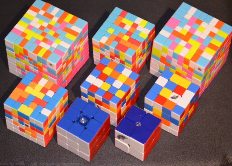
So I took the bull by the horns and learned a method to solve virtually any cube. It’s quite simple when done right but requires some persistence and trial and error at the beginning. I’ll probably make some video tutorials even if there are already many of them out there. The method I use enables me to go from this:
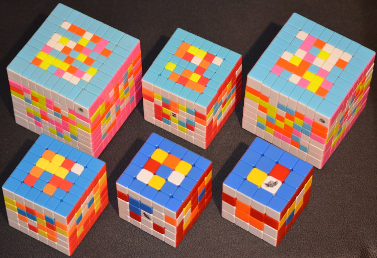
to this where the 2×2 and 3×3 have been solved and the others are on the way:
to finally all of them solved:
And those don’t have stickers, no cheating allowed and I wouldn’t paint them and ruin them.
There are many methods to solve cubes. Fast ones, especially for the 3×3, that don’t really work for other cubes. Universal and slow ones.
My goal was to solve any cube, including my wife’s present, not to do what is called “speed cubing”. I actually wanted to learn as few “algorithms” or “formulas” as possible as I don’t plan to solve cubes for the rest of my life. I reduced it to:
2 algorithms for the 2×2,
2 more algorithms for the 3×3 (that’s 4 in total),
3 more algorithms for the 4×4 and all others (7 algorithms in total).
Yes, you read that right: with as little as 7 “programmed series of moves”, you can literally solve *any* cube.
Most of these “algorithms” are easily memorized using mnemonics such as a little story. It is also necessary to be able to perform the mirrored version of every algorithm, but that’s not a big deal with a little training.
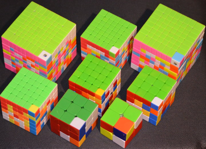
Here are the basic steps to solve all these cubes. First solve the center part of a single face (here the green one), this doesn’t need any algorithm as it is quite simple (note that nothing needs to be done for the 2×2 and 3×3):
Next, solve the edges of that face, making sure that the other sides match the colors of the centers of the other sides. No need for an algorithm here either, it is quite intuitive. However, for cubes with an even number of pieces, you have to memorize the order of the colors, clockwise red, white, orange, yellow. Just use whatever mnemonic works for you. If RWOY, like in “Rob Rwoy” works, then that’s what it is. 🙂
Note how it forms a cross on top of the cube (again except for the 2×2 which still doesn’t change).
Then solve 3 of the green corners on all cubes, which is very easy and simply requires a bit of logic:
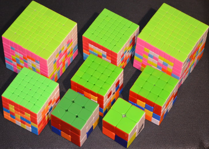
Let’s turn all the cubes to the side to have a better look at what happens next:
Start solving the edges from the green corners (see how the edges that are closer to us in the picture start getting solved), this again doesn’t require any algorithm:
Let’s turn the cubes again:
Now solve the last edge and solve the half edge under it as well as other edges that may not have been finished yet. Here comes the first algorithm:
Note that at this point, the 2×2 is half solved and 2/3 of the 3×3 is solved as well. Let’s turn the cubes to their other side, where everything will happen from now:
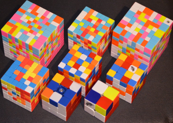
At this point, the 4 blue corners can be solved with 3 different algorithms (one of them is a combination of two others, so it doesn’t count as new), and the middle blue edge is also solved with one algorithm. At this point, the 2×2 and 3×3 are solved. So it looks like this:
Now let’s solve the remaining top edges (blue ones) with one algorithm:
Note that the edges of the second row from the top are still not solved, so now is the time to solve them, one algorithm is required for this:
And now, the centers need to be solved with one single algorithm declined in different ways, it is generally the longest part, especially with bigger cubes, and needs some planning, memory and solving skills. Et voila!
Stay tuned for some videos in the future that will show how to learn and apply the different algorithms.