There is a lot of material available in French on the original Galileo Module, which I already translated into English. But because I believe it is important to spread the information to other places than French-speaking communities, I am releasing my own version of the Galileo Module in English. This version will also explain to the reader the basics of the Relative Theory of Money so that no prerequisite is needed to read this blog article. This first part addresses the first part of the Galileo Module about changing frames of reference in a libre currency.
What is a libre currency?
A libre currency as defined by M. Laborde in his Relative Theory of Money (which I will shorten to “RTM”) is a currency in which all individuals in an economic zone create money equally and at regular intervals. The amount of money created by all individuals is always a fraction of the existing money mass and every single individual at a given time creates exactly the same amount of money as the others. Thus, money is no more created by central entities, or banks, but rather by every living human, in full symmetry with his peers at a given time but also across generations. This is perfectly possible today thanks to blockchain technology. It is no coincidence in my opinion that the RTM was published in 2010, after the 2000 and 2008 crises but first and foremost shortly after the invention of the concept of blockchain in 2008.
(a) Changing Frames of Reference in Space
The spreadsheet for this part can be downloaded here.
Libre currency
We need to build a spreadsheet for the amount of libre money created by 3 individuals, I1, I2, and I3.
As explained above, libre currency functions as follows: regularly, every individual in the economic zone creates a share of money. This share of money is called a “Universal Dividend”. So at every interval, we need to calculate the total amount of money in circulation and multiply it by a celerity factor called c which is the percentage of the Universal Dividend. The result must then be divided it by the number of participants to get the Universal Dividend per person.
Note that the interval can be chosen randomly, but the shorter the better. In the current libre currency Ğ1 it is every day, but in this publication, we’ll stick to every year otherwise the spreadsheets could be quite huge!
The Absolute Reference Frame (counting monetary units)
Here is the beginning with 3 individuals I1, I2, and I3 who start in life with very different values in their accounts:
Year
|
I1 |
I2 |
I3 |
N |
Total |
Total/N |
UD |
c |
| 0 |
0 |
10 |
100 |
3 |
110 |
36.67 |
3.67 |
0.1 |
- N is the number of individuals
- Total is the total amount of money available also called Money Mass, here it is simply the sum of the money of I1, I2, and I3
- Total/N is the average amount of money available per individual
- UD is the Universal Dividend per individual, which is Total / N × c
- c is the celerity of the monetary creation, the percentage at which new money is created, here it is 10%=0.1. This means that the money mass will grow by 10% every year. Note that c cannot be chosen completely at random since it depends on the life expectancy of the population. 10% is an acceptable value for a population whose life expectancy is roughly between 35 and 80 years. For a population with an average 80 years life expectancy, the RTM predicts that values for c should be chosen between 6 and 10%.
At year 1, every single individual will create exactly one UD:
| Year |
I1 |
I2 |
I3 |
N |
Total |
Total/N |
UD |
c |
| 0 |
0 |
10 |
100 |
3 |
110 |
36.67 |
3.67 |
0.1 |
| 1 |
3.67 |
13.67 |
103.67 |
3 |
121 |
40.33 |
4.03 |
|
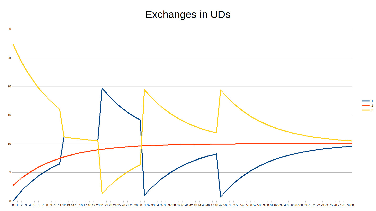
We note right away that I1 has gone from 0 to 3+ units, while I2 sees a 30% increase of his money and I3 sees only a 3% increase in his money. The money mass is also growing which means that the UD for the next year is growing as well.
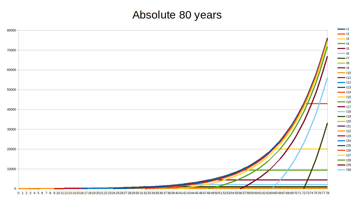
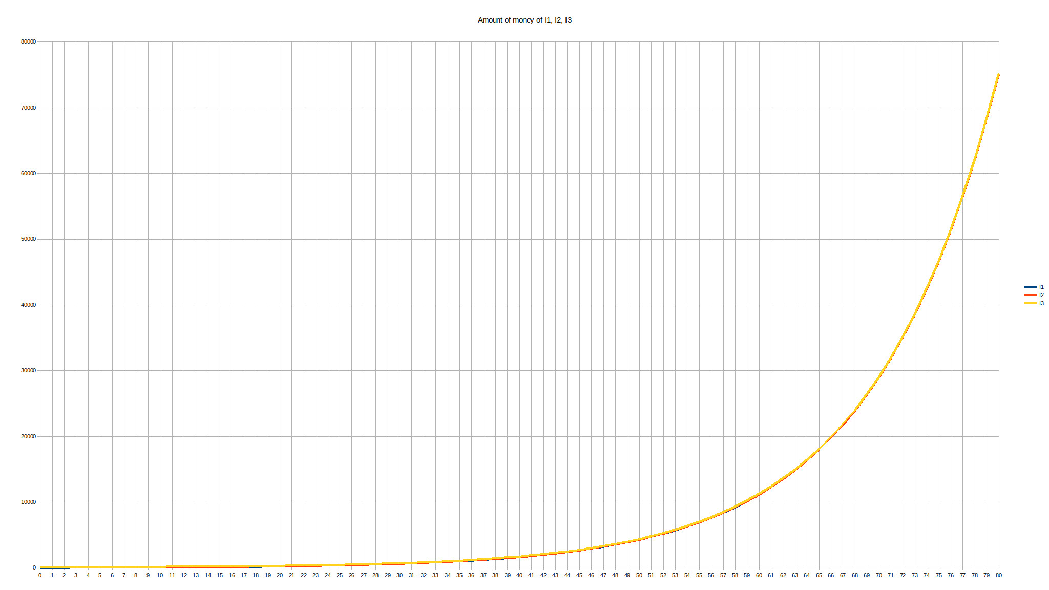
Because we are not computers I will stop showing the spreadsheet and show graphs instead which are much easier to read. Here is the graph of the amount of money over the first 20 years:
Unsurprisingly, this is an exponential curve. We can see that, over time, I1 who was the poorest, as well as I2 who was relatively poor compared to I3, are “catching up” with the richest – who still remains the richest. Now let’s extend this to 40 years, which is currently a half-life of a Westerner:
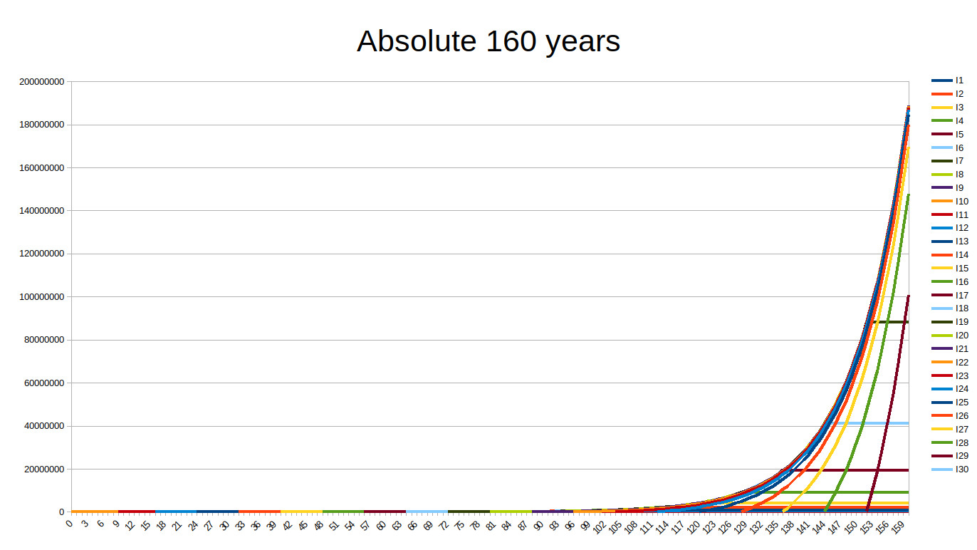
This time, it gets more difficult to see the difference between I1 and I2, and they are definitely catching up with I3. Let’s extend that to a full 80 years of life:
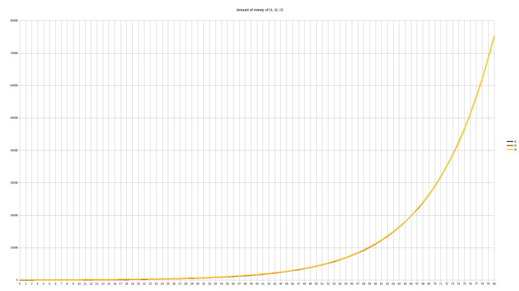
This time, the three curves are impossible to distinguish.
At first sight, this graph can be quite scary when we speak about money, especially about the total money mass. This reminds us of the Zimbabwe Dollar where an exponentially growing money mass is accompanied by exponential inflation, which is never a good thing when a state starts printing money like a crazy gambler:

The Relative Reference Frame (counting in proportion of the money mass)
Instead of counting monetary units, let’s change the frame of reference and use the percentage of the money mass as a reference.
Let’s go back to the first year of our 3 individuals and count how many percents of the existing money they possess:
| |
Year
|
I1 |
I2 |
I3 |
| Absolute |
0 |
0 |
10 |
100 |
| Percentage |
|
0 % |
9.09 % |
90.9 % |
I1 has 0%, I2 has 9% and I3 has 91% of the total monetary units.
We have seen that in year 1 the amount of money they have has changed quite a bit:
| |
Year |
I1 |
I2 |
I3 |
| Absolute |
1 |
3.67 |
13.67 |
103.67 |
| Percentage |
|
3.03 % |
11.29 % |
85.67 % |
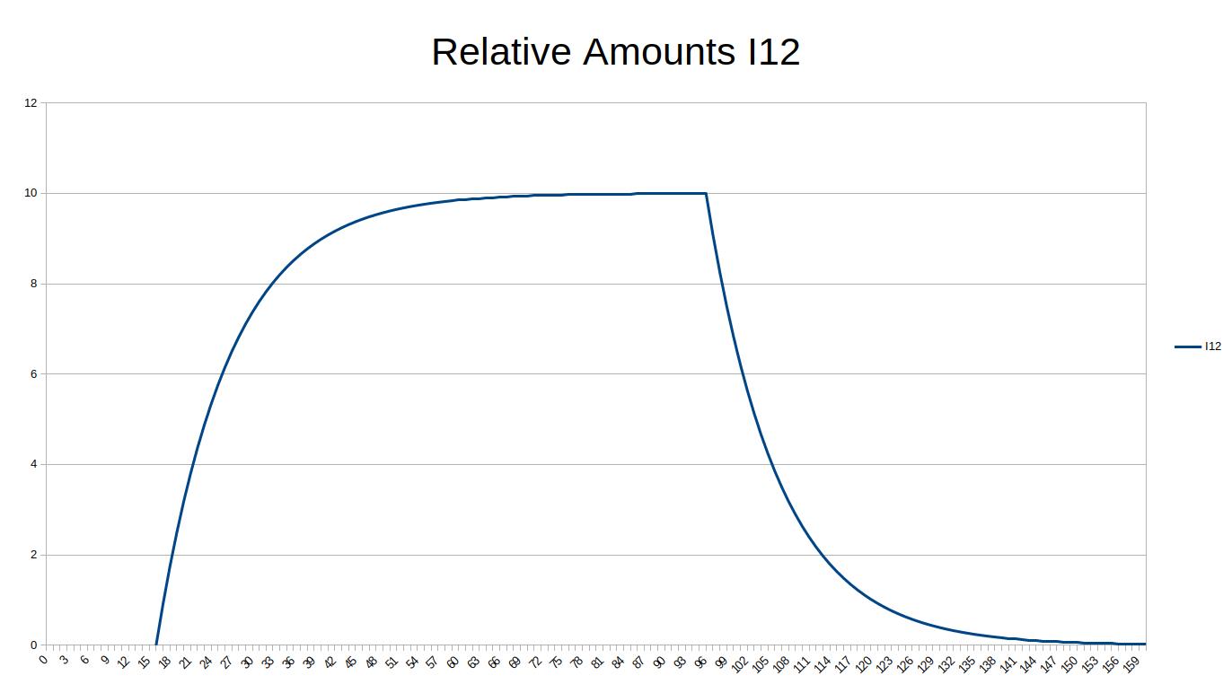
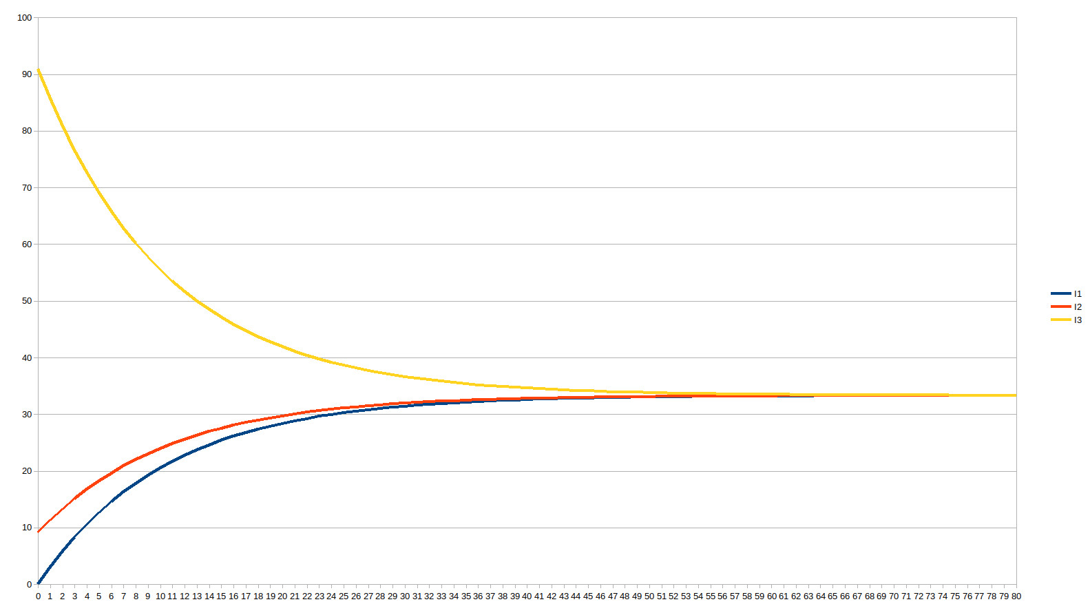
Now instead of representing the charts with the monetary units, let’s draw the chart for the percentage of money they own over time and during 80 years:

It is now very clear that I1 and I2 are getting a higher percentage of the money over time, at the expense of I3. All accounts are mathematically drawn towards the mean of all accounts.
We can already note that they approximately reach the mean after 40 years. This is because we have chosen the celerity to be 10%. Let’s see what happens when we choose 6% instead of 10%, as those are the bounds specified by the RTM for a life expectancy of 80 years:

This time, the mean is roughly reached only after 80 years, which is totally in sync with the predictions of the RTM: the highest recommended values of c cause accounts to converge within a half-life, while lower values of c cause accounts to converge within a full life.
We will now stick with the value of c = 10% in the rest of the article.
Both the graph in relative value and absolute value can be translated into references where the sum of all money is 0 at all times. In other words, at every moment, we check the difference between every account with the average total money per individual instead of the actual amount.
In this reference frame, the quantitative graph is quite surprising as it basically doesn’t move at all. Indeed, the absolute monetary difference between the individuals doesn’t change. It is proportionally very different when you consider the total money mass, but in absolute values, it never varies since we consider that our individuals give exactly as much as they receive (either because they don’t make exchanges at all, either because their exchanges are perfectly balanced):

On the other hand, the relative frame does show the shrinking differences between the three since it takes into account the percentage of money that each of them possesses:

Note that in this frame of reference, we have suddenly lost all thought of “hyperinflation” that could have worried us in the absolute frame of reference. After all, this is a very stable way of creating money!
Taxation
Now that we’ve studied what happens with a libre currency, let’s check what happens when we apply a fully proportional tax, eg. we take a fixed rate of tax on the accounts, calculated that way for an account R(t):
tax(t) = c × (R(t) + 1) / (1 + c)
The total collected tax is then redistributed equally among every single individual.
Let’s calculate the tax for the first year:
| Year |
I1 |
I2 |
I3 |
Total |
T1 |
T2 |
T3 |
Total Tax |
c |
| 0 |
0 |
10 |
100 |
110 |
0.09 |
1 |
9.18 |
10.27 |
0.1 |
We can right away note that the tax on the rich is higher than the tax on the poor, which is normal since it is proportional. But we also note that there is an anomaly during the first year because the poorest has 0 and cannot be taxed. So we’ll adjust this special case to be 0 (is that fair – should he pay a tax to cover for this later?…). Now let’s see how it evolves over the next few years:
| Year |
I1 |
I2 |
I3 |
Total |
T1 |
T2 |
T3 |
Total Tax
|
c |
| 0 |
0 |
10 |
100 |
110 |
0 |
1 |
9.18 |
10.18 |
0.1 |
| 1 |
3.39 |
12.39 |
94.21 |
110 |
0.40 |
1.22 |
8.66 |
10.27 |
|
| 2 |
6.42 |
14.60 |
88.98 |
110 |
0.67 |
1.42 |
8.18 |
10.27 |
|
| 3 |
9.17 |
16.61 |
84.22 |
110 |
0.92 |
1.60 |
7.75 |
10.27 |
|
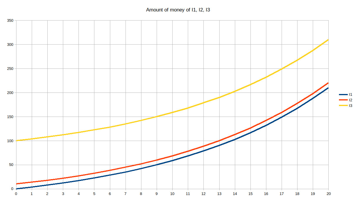
We see that we take the same amount of taxes every year (10.27) except the first year because of the anomaly of I1. Globally, the trend seems to be the same as in libre money: all accounts seem to tend toward one another. Here is the chart when counting monetary units:

As predicted, the accounts all converge towards the average. But note that this is the graph in absolute values now, whereas in libre money the quantity of money was growing exponentially. Now let’s have a look at the graph in relative values:

Unsurprisingly, it does look the same, the only change being the scale.
So the big surprise (or not!) here is that libre currency is equivalent to a certain form of tax redistribution. The pleasant surprise with tax redistribution is that we don’t need to “burden” ourselves with the relative reference frame since the quantitative reference frame with tax redistribution is already behaving the same way as the libre currency.
Let’s proceed and collect taxes for our perfect redistribution system and put the RTM in the trash can! (humor – read on!)
Thoughts on taxation systems
Let’s have a look at tax collecting systems and their efficiency in the history of mankind.
If you dig just a little, you’ll find that tax evasion today is absolutely everywhere. It is said to leak more than 1,500 billion (yes, 1,500,000,000…) dollars every year in Europe alone. Besides, there is “illegal” tax evasion, but there is also “legal” tax avoidance which, thanks to the very lenient tax laws in many countries, allow the richest to avoid paying much taxes. The funniest part is that the French government is definitely not looking at big tax evaders, but looking instead at petty and insignificant tax evaders. They are really not seeing the elephant in the room!
This is actually not new. Tax evasion has been around for a while, actually at least since late Antiquity (2 different links).
In Ancient Greece, they actually found an original way of fighting tax evasion. Should we, too, incentivize our richest citizens to pay taxes in order to be revered and adored as benevolent philanthropists? Well, they already found the trick around that so it seems to be quite useless nowadays.
Let’s ask a simple question: why has tax evasion been always so popular? It is easy to explain: human nature is such that we hate to lose something, which is the case with taxes. On the other hand, creating money is always winning something so it is much easier to accept, even if you are actually losing in proportion!
Oh well. Let’s dig back the RTM from the trash can and read it one more time. 😀
Libre currency vs tax redistribution first and last round
The huge advantage of a libre currency compared to a tax-collecting system is that there is no avoiding taxes and their redistribution, which is then simply carried out mathematically through monetary creation. Ingenious!
Part 2 is a little bit technical so if you’re not into technicalities about computers, you should skip directly to Part 3.

 Hmm, it doesn’t look as stable as we thought. Someone in the US who would buy gold in early 1980 thinking that this thing is definitely going up would absolutely be astounded to see he has lost half of the value 2 years later compared to the USD. Of course, the one who bought gold in 1975 with USD would probably have been very happy to sell his gold to get back some USD in 2012 (x10!).
 Oh, it seems silver is even more unstable than gold compared to the USD. What about this rare metal called Palladium?
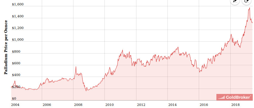 Well, it’s not so different. Okay, maybe it’s the dollar that is not stable?
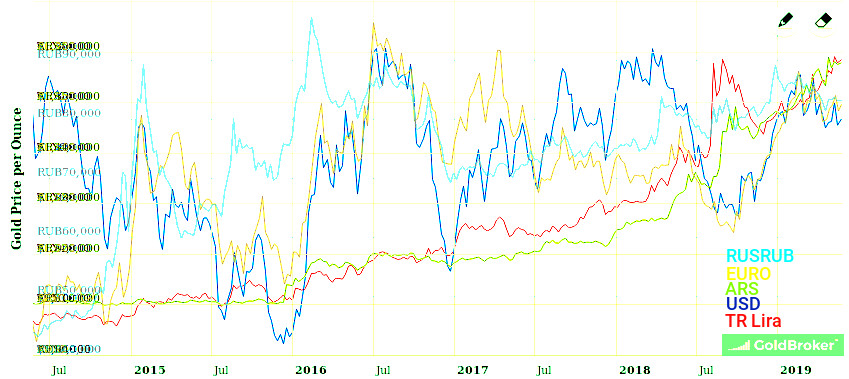 What a Christmas Tree! This is total nonsense! Especially in July 2018, are we supposed to think that gold is “going up” or “going down”???
 The truth is that nothing is going up or down by itself. Values are always “going up” and “going down” compared to another value. So these variations are totally normal, as nothing has such a thing as “intrinsic value”. Objects have “properties” that are then valued by humans to be “better”, “similar”, “worse”, than other properties of other objects. Gold is rarer than silver? Maybe that’s a reason why it’s valued more. But isn’t it also “better” because it doesn’t get oxydized while silver does? On the other hand, gold is “soft” and can barely be used in its pure state. Silver, on the other hand, is a hard metal, isn’t it better then? See, there are many things that drive the “value” in our minds of one thing, even if it seems simple. But it is always “relative to something else”. A hunter-gatherer tribe will have no business with you if you try to give them a golden bar, they can’t eat it! But for sure, they absolutely could use that big axe you have in your hand to hunt game, so they will value that axe much more than your gold bar.
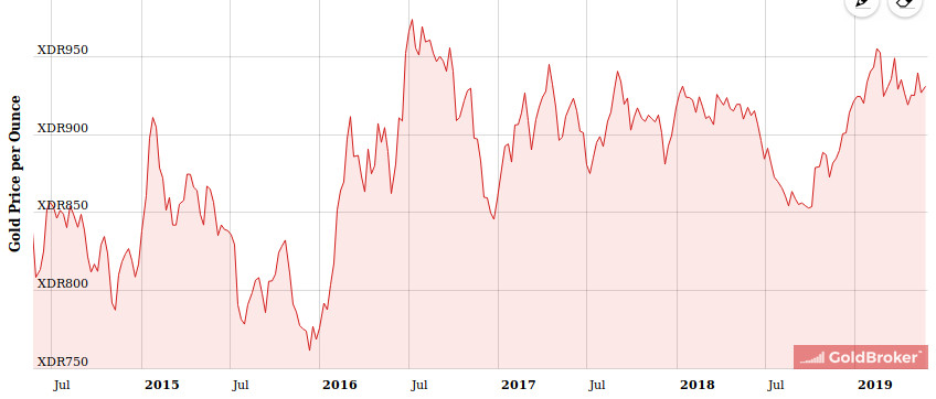 Unsurprisingly, it bears a resemblance with the charts involving the USD and EUR. But still not stable, which we know now is quite normal.
 In fact, the price of a Parisian flat seems to be quite stable compared to M3, which is the total amount of euros in circulation. Surprisingly enough, it is even plummeting since 2011!
 That’s not cool, the price of a Parisian flat lost almost 20% since the 1990s compared to gold. Surprised? I’m not.