The Relative Theory of Money – English Translation of the Leibnitz Module

This is the translation of the Leibnitz Module of the RTM, which follows the Bresson Module.

Leibnitz Module

(a) Thoughts on the Relativity of Prices (N)

Let’s assume that for a short time compared to life expectancy (a few years), the prices of some known values are relatively stable in the M/N frame of reference. Given this hypothesis, simulate:

  • create the spreadsheet of a Libre Currency in both Quantitative and Relative (UD) frames while the population is composed of N individuals
    including I1, I2 and I3 ; N is a variable represented in a column, during 80 years, one line per month (80×12 lines) as well as a newcomer I4 who enters when N varies,
  • on a short period of time, express the relative price in the frame M/N during a few years of an economic value V ; translate the quantitative price in UD,
  • express during the same period the price of V compared to the accounts of every individual,
  • simulate cases where “N increases strongly” and “N decreases strongly” in a few years, create the charts of the prices of V (which remains quite stable in the quantitative frame), in the 3 units as well as relative to the 4 individuals,
  • Compare and interpret the results.

(b) Reflections on the formula of the UD when N is unstable

  • In the same spreadsheet, simulate two strong local variations of N (10 times growth/reduction) during a small period of time (2 years), N remains stable otherwise,
  • add I4 who is a newcomer during the variation of N,
  • express for the 4 individuals the variations of the price of V (which we will assume is still stable in the quantitative frame) in the 3 units (quantitative, UD, M/N) and relative to the accounts of each individual, during a period of 20 years around the variations of N (before and after),
  • try to find a possible range for the UD’s formula between minimal and maximal values by studying the case of the 4 individuals,
  • Compare and interpret.

(c) Studying different UD formulas

  • In the same spreadsheet, simulate two strong local variations of N (x 10) on a short period (2 years), N remains stable otherwise,
  • Simulate for the 4 individuals different formulas for the UD that can be studied in a 20 year interval before and after the variation of N,
  • simulate the same formulas when N is stable in another spreadsheet,
  • compare each formula graphically by comparing it to M/N when N is stable,
  • calculate for each of these formulas the standard deviation with the stable case,
  • Compare and interpret the results.

(d) General interpretation on relativity

(e) Conclude the publication

My Yolland Bresson Module – Part 2

Welcome to the second part of my version of the Yolland Bresson Module, started in Part 1.

(d) Exchanging values during 50 years in a Libre currency

In this part, we’ll see what happens when individuals do some exchanges, since it is actually what money is here for! So we’ll have generations of 10 people which replace each other over time and watch the impacts on the accounts of these exchanges over time.

Simple exchanges

To begin with, the sample given in the Module is to have exchanges at 5, 15 and 30 years. Besides, in my sample, I’ve given a very unfair distribution to my individuals with the oldest having a lot of money while the youngest has 0. I also chose to use the relative scale for the exchanges so that we can actually compare the relative amounts which don’t change over time, with an average of 10 UDs for all individuals. Finally, the amounts that are exchanged are quite big, making the individuals’ accounts switch from “rich” to “poor” and vice-versa at every exchange:

Year I1 I4 I5 I7 I11
5 -10 UD   10 UD    
15   -8 UD   8 UD  
30       -10 UD 10 UD

Just for the record, this corresponds in the absolute scale to the following exchanges:

Year I1 I4 I5 I7 I11
5 -72.47   72.47    
15   -150.4   150.4  
30       -785.2 785.2

As expected, the same amounts in UD correspond to exponentially growing numbers in the absolute scale.

Visualizing the impacts of simple exchanges

Unfortunately, the absolute graph doesn’t show anything because of the exponential curve, so we’ll directly switch to the log view:

While we do see the exchanges, they seem to have extremely little impact on the overall curves. Consequently, let’s switch to the relative scale:

What happened is pretty obvious now: although they have exchanged very big amounts of money, in the end the result is that when they die their accounts converge toward 0 and new generations (after a few decades) are not impacted by what has been done by the previous generations. Therefore, these new generations can choose their own path and their own values, regardless of what their parents have done and valued.

Focusing on one individual

We can also have a look at the account of one of them only, for instance I7 who has done two transactions:

Obviously, because he has gained quite a bit at year 15, his account has inevitably decreased in relative terms after that compared to other accounts so that all of them reach the mean of all accounts. But then as he becomes “poor” at year 30, his account starts tending toward the mean again, this time by “growing”. And of course, as death takes him away, his account tends toward 0, as everyone else (except for vampires of course).

Double accounting

Until now, we have only considered transactions between humans, who generally exchange money to compensate another exchange in real life: buying some object or service. However, we could express that in a “double-entry” table for each individual where we don’t consider only monetary exchanges:

Year I1 – Credit I1 – Debit
5 +motorcycle -10 UD

With that in mind, we can actually fill the previous table with the double accounting for each event and each individual:

Year I1 I4 I5 I7 I11
5 -10 UD
+motorcycle
  10 UD
-motorcycle
   
15   -8 UD
+boat
  8 UD
-boat
 
30       -10 UD
received coaching
10 UD
spent time coaching

Obviously, every monetary exchange has its own counterpart in the “real world”, either by transferring the property of something from someone to someone else, either by giving one’s time/expertise/work, whatever you call it, to someone else.

Double accounting – including the UD

In the meantime, there is really something missing in this table. In the balance of every individual’s account, a Universal Dividend is created every year. For everyone of them. So if we forget about their exchanges, the balance sheet is somehow missing something:

Year I1 I4 I5 I7 I11
5 +1 UD +1 UD +1 UD +1 UD +1 UD
15 +1 UD +1 UD +1 UD +1 UD +1 UD
30 +1 UD +1 UD +1 UD +1 UD +1 UD

Think about it, isn’t there something missing? We have UDs that are added, but nothing is subtracted to make the sheet balanced.

Year I1 – Credit I1 – Debit
5 +1 UD ???

Or is it really so?

The counterpart of the UD

Well, it isn’t. Every one of us is alive and is somehow always doing “something”. During our life, we give our time and energy to things that are meaningful to us. In addition, sometimes without even noticing it we create value in society, even in the smallest acts of our lives.

For instance, say you watched a football match yesterday while drinking beer and eating junk food. That doesn’t seem much of a contribution to society. I actually don’t like football, if you ask me, you’ve wasted your evening, and wasted yourself with the alcohol as well!… 😀 the fact is that my opinion here is not relevant since here we’re interested about you.

Due to the match you watched, maybe the next day at work you’ll have a nice chat with your colleagues and somehow, with that simple chat and some jokes about the match, you’ll have created a relaxed atmosphere at work that will make everyone positive for the next few hours. Isn’t that a contribution after all? Frankly, do you really think that brightening the day of someone else is a waste of your time?

Furthermore, it gets even more interesting if you produce some “things” that are not recognized by your peers (or even by yourself!) but that may be recognized as great achievements in the future, such as Mozart’s compositions or Vincent van Gogh’s paintings. As we’ve already seen in the Galileo module, we can call these ğvalues. We may not all be geniuses, but we all make contributions that are not recognized today as full “values”, and which have the potential of becoming values in the future.

Furthermore, other people in another part of the Earth might also be interested in your creations because the cultural biases of another society will be able to recognize them as values, while the society you live in don’t recognize them as values – think for instance metaphysical, meditation-related discoveries that would be considered utter b**lshit in the West but greatly valued in the East.

Let’s fill the blanks

With that in mind, let’s get back to our table. We can now fill it with the appropriate negative accounts of your time that you spend being alive and contributing to society as a whole by focusing on your own values and creating ğvalues:

Year I1 I4 I5 I7 I11
5 +1 UD
-ğvalues
+1 UD
-ğvalues
+1 UD
-ğvalues
+1 UD
-ğvalues
+1 UD
-ğvalues
15 +1 UD
-ğvalues
+1 UD
-ğvalues
+1 UD
-ğvalues
+1 UD
-ğvalues
+1 UD
-ğvalues
30 +1 UD
-ğvalues
+1 UD
-ğvalues
+1 UD
-ğvalues
+1 UD
-ğvalues
+1 UD
-ğvalues

Hurray, we do have a balanced double-accounting sheet now.

In conclusion, we have filled the double-entry table and everything is balanced now, thanks to the notion of ğvalue, which is the counterpart of the UD.

Multiplying exchanges

I have also played a little with more exchanges.

Here is the graph of many exchanges made by the exact same individuals:

Ok, I’ll have to agree that it’s quite messy. However the first thing we can notice is that, although they did make a lot of very unbalanced exchanges, the conclusion is always the same: whatever they did, their accounts never became excessively high (up to 2.5 times the average of all accounts) and they always go back to 0 after their death.

Nevertheless, these exchanges are not random – let’s detail what happened here in more detail.

Hoarding “things”

There are many questions that arise about Libre Currencies. One of them is the fact that people would be tempted to get away from their money and buy “something” that would be a store of value for them (think “gold”, for instance). Then later, by selling those things back, they would have an advantage since they wouldn’t have lost their purchasing power, unlike storing libre units of value which statistically lose value exponentially in time.

I have simulated exactly that with one individual, I10. During the first part of his life, he systematically spends his money to buy things. After that, as he reaches his 59th birthday, he sells those things back. Note here that I have considered that the price of those “things” he bought have not changed in the relative scale. For instance, that could be true for something like gold, but you could also imagine many other things. I have isolated the graph for this individual and the people he exchanged with:

It is apparent here that he seems to be “cheating” during the first part of his life. Obviously, he refuses to go to the mean of all accounts so his account gets always filled with money, while other people’s accounts get higher.

Conversely, toward the end of his life, by selling what he has been hoarding during his whole life, he suddenly becomes very rich compared to the others, while everyone else is getting poorer.

Thoughts on I10

Obviously, this technique could be used to “optimize” your account in Libre Currency. I have seen people do that during Ğeconomicus games. However, this technique did not seem to be as fruitful as it could appear at first sight. That is because as the person is “buying” things he is actually not using, he is depriving himself of a very important tool: money itself. In other words, instead of using money for what it is, a means of exchange, he is using it for hoarding things, therefore giving himself a penalty because he cannot exchange with money much anymore.

Furthermore, he takes a great risk. Who knows if the “things” he bought will be considered as having any “value” at all in 30 years when he plans to sell them back? Nobody can guarantee that. Therefore, he’s taking a big chance, and may find himself with no money in his account and be surrounded with useless objects that nobody wants to buy. Certainly, that was not a very smart move! Besides, he could be having problems if he bought a lot of similar things: as he is selling them back, their price will inevitably get lower.

Additionally, we can also wonder how much of those “things that are stores of value” he will be able to buy, as everyone else will also value those things as such. So there will inevitably be a balance to be found on the prices of those objects, while money is circulating around, which is exactly what it was invented for!

Finally, although I10 did manage to get richer somehow toward the end of his life, he did not get “insanely” rich. So such a scheme is not a huge problem overall as he has paid a strong penalty for the rest of his life.

Inheritance

Another interesting question is the one of inheritance. Therefore, I have simulated a family that would try to transmit its monetary riches to its descendance in the hopes of getting richer and richer, as it happens with today’s monetary system. Indeed, despite all inheritance taxes and efforts by the State to grab whatever it can, the rich manage to get richer, generation after generation.

Without further ado, here is the graph of the “inheritance scheme” family who pass on the wealth to the spouse then to the children when one of their member dies:Indeed, they do manage to get a little richer than the average, thanks to the inheritance. Let’s say maybe twice as rich on average. Undoubtedly, that’s absolutely ridiculous compared to the rich today who are millions of times richer than the average population. Besides, everyone else will probably do the same thing, so there is no inequality here. The main point here being that even if trying to pass on great wealth, nobody can get hundreds of times richer than the others.

(e) General interpretation on Relativity

As a conclusion, we have first seen that in a Libre Money system, everything has its own counterpart: the UD is balancing the ğvalues created by humans.

Besides, this balance ensures that no minority manages to tip the scale in their favor since everyone’s contribution is always pushing the global scale to be symmetrically balanced in space and in time as well.

My Yolland Bresson Module – Part 1

Here is my version of the Yolland Bresson Module which follows the Galileo Module.

As the data has already been gathered in the last part of the Galileo Module, we can switch directly to part (b) and create the charts. Note that I based most of my data on the spreadsheet by Inso. I’ve added to it most of the data since 2014 until 2019.

(b) Create Relative Charts

In the Galileo module, I have already discussed the price of gold over time especially compared to different currencies and even compared to real estate prices in Paris.

The Gold Standard effect

One very interesting graph is the long term one which compares the USD to gold:

This is an unusual graph in which we observe the purchasing power of the USD compared to gold. The two steps of the gold standard, before and after 1929, are clearly visible. Then in 1971 as Nixon breaks the gold standard, the fall of the dollar compared to gold. One could say that, by forcing the gold standard, officials have tried the impossible: forcing one value to be equal to another one, although those values were appreciated quite differently in people’s minds.

The point here is that we can always compare any value to any other value, and no value stays equivalent to another one over time.

Looking from another perspective

We always look at prices “in euros” or “in dollars” but we never compare random values together, such as real estate and welfare.

So let’s do this just now and draw the chart of real estate prices expressed in units of welfare!

We’ve seen in the Galileo module that if you own gold, then the price of a flat is actually going down since the 1990s. But if you’re on welfare, the price has more than doubled in the same period of time.

(c) Charts

The point of this part is to look at prices not only over time, but also across geographical regions. Cuckooland has done a tremendous job which allows to see the prices of real estate change over time as the raise in price clearly starts in the center of the Capital, and diffuses first to the West (the richest suburbs) then to the rest of the area. Play with it, it is excellent! He has also rewritten some of it into a new app which he even translated to English. It is also available as a block. Enjoy!

Real Estate around the World

This is all about Paris. But what about the rest of the world? Are real estate prices all going up? You can download the spreadsheet real-estate-world.

Here is a chart of real estate prices worldwide since the early nineties, gathered from the IMF.

Obviously, some prices are going up, but some others are going down!

The geographical changes are also not uniform at all. For instance, in the UK, the prices between the London area and the rest of the UK are absolutely not following the same trend:

While London prices are skyrocketing, doubling between 2005 and 2019, prices elsewhere are not that crazy.

Wheat prices in the US

There are many other interesting values to be considered when it comes to geographical differences.

You may think that prices of wheat, for instance, are pretty much the same everywhere. Well, they are definitely not. The spreadsheet for this is available for download wheat-us. Here is a chart of wheat prices in the US over time:

From Denver to Portland, there has been a point in 2017 when you would pay double the price of wheat in Portland compared to Denver. I’m no expert in wheat crops in the US, but obviously Denver is a big producing area while Portland is not as big.

One other apparent trend here is that prices have diverged during mid 2016 and are getting closer again at the beginning of 2018. Many factors can explain this, such as a bad harvest which is actually confirmed for 2016. When the area already produces very little, a bad harvest means you may even need to import some wheat from elsewhere. But for a big producer, it has less impact. Although it may affect your exports, you still have more than enough locally.

Now that we know that we can actually compare any value with any other, we can actually compare the wheat price in Portland to the Denver price and create the corresponding chart:

We see here that Portland paid an immediate toll for the bad harvest in 2016 and only recovered in mid 2018, 2 years later.

Conclusion

Every value evolves with time, but also in space, always relative to other values. Many factors drive these changes: geography, climate, natural resources, social bias and trends of values in society, individual preferences, etc.

That’s it for Part 1, I will continue in part 2.

The Relative Theory of Money – Yoland Bresson Module Translated to English

Following the Galileo Module, the Yoland Bresson Module is the second module proposed to go deeper in the RTM. Here is a translation of the module in English.

The Yoland Bresson Module

(a) Get some data in a spreadsheet

The data has already been gathered during the last part of the Galileo Module:

(b) Create charts

Long term graphs of: Gold/$, Silver/$, Silver/Gold, Gold/€, Silver/€, Gold/M3€ , Silver/M3€, Gold/JSI-Welfare, Silver/JSI-Welfare.

Create the reverse graphs ($/Gold, $/Silver, etc.).

(c) Charts on Real Estate

Real Estate prices in Paris vs €, Gold, Silver, JSA/Welfare, M3€.

Same charts with real estate prices in another location, preferably a low density populated area.

Animate the results on a map with time. Change the reference frame (rather than €, use Gold, Silver, or any other reference frame).

Compare and discuss the results.

(d) Exchanging values during 50 years in a Libre currency

  • Create spreadsheets in absolute and relative frames for 30 individuals I1-I30 during 160 years.
  • Simulate large exchanges at t1=5 years, t2=15 years and t3=30 years,
  • Discuss numerical values as well as graphically, using double-entry accounting (think about Ğ(x) – eg. values that are not monetized because they are not recognized as values),
  • Summarize your thoughts about how humans, values and money, flow with time.

(e) General interpretation on Relativity

The next module is the Leibnitz Module.

My Galileo Module – Part 5

Here comes the last part of the Galileo Module: the relativity of values.

The aim of this module is to understand that no value is absolute, and that all values are relative to one another.

(e) Establish long term relative variations of different values

Metals

First I will study the price of gold, which we all now for sure is one very stable reference, right?

Let’s have a look at this very stable value:

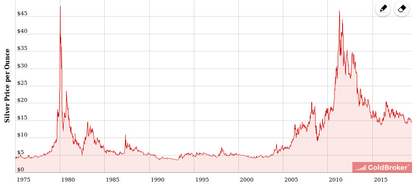
Hmm, it doesn’t look as stable as we thought. Someone in the US who would buy gold in early 1980 thinking that this thing is definitely going up would absolutely be astounded to see he has lost half of the value 2 years later compared to the USD. Of course, the one who bought gold in 1975 with USD would probably have been very happy to sell his gold to get back some USD in 2012 (x10!).

But enough of the Gold. Silver must be probably better than gold, and reassure us on the fact that those metals are very stable in value:

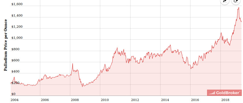
Oh, it seems silver is even more unstable than gold compared to the USD. What about this rare metal called Palladium?

Well, it’s not so different. Okay, maybe it’s the dollar that is not stable?

Holly Gold

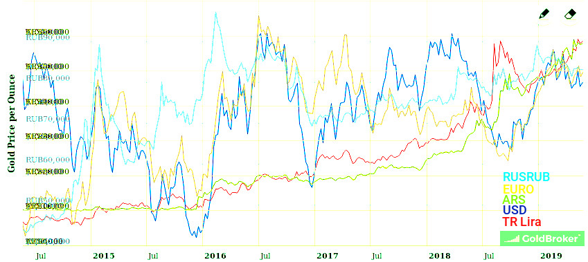
Let’s have a look at Holly Gold compared to different currencies:

What a Christmas Tree! This is total nonsense! Especially in July 2018, are we supposed to think that gold is “going up” or “going down”???

The truth is that nothing is going up or down by itself. Values are always “going up” and “going down” compared to another value. So these variations are totally normal, as nothing has such a thing as “intrinsic value”. Objects have “properties” that are then valued by humans to be “better”, “similar”, “worse”, than other properties of other objects. Gold is rarer than silver? Maybe that’s a reason why it’s valued more. But isn’t it also “better” because it doesn’t get oxydized while silver does? On the other hand, gold is “soft” and can barely be used in its pure state. Silver, on the other hand, is a hard metal, isn’t it better then? See, there are many things that drive the “value” in our minds of one thing, even if it seems simple. But it is always “relative to something else”. A hunter-gatherer tribe will have no business with you if you try to give them a golden bar, they can’t eat it! But for sure, they absolutely could use that big axe you have in your hand to hunt game, so they will value that axe much more than your gold bar.

XDR

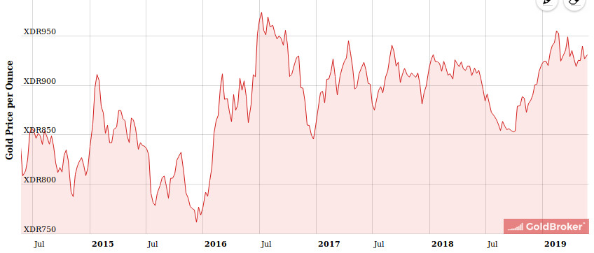
Next, let’s see the value of gold compared to something that is a worldwide reference: the SDR (code XDR), Special Drawing Rights. Never heard about it? It’s a world currency, a basket of different currencies (USD, EUR, GBP, JPY, and more recently CNY). Here is the chart:

Unsurprisingly, it bears a resemblance with the charts involving the USD and EUR. But still not stable, which we know now is quite normal.

Real-Estate in Paris

We all know (especially French people) that the prices of houses and flats in Paris is surging for the last decades. Unfortunately, it may be true when counting in units of euros, but if we compare the prices to the total number of euros in circulation, let’s see what happens:

In fact, the price of a Parisian flat seems to be quite stable compared to M3, which is the total amount of euros in circulation. Surprisingly enough, it is even plummeting since 2011!

Last but not least, let’s compare the price of a Parisian flat if we were to buy it with Gold:

That’s not cool, the price of a Parisian flat lost almost 20% since the 1990s compared to gold. Surprised? I’m not.

Conclusion on the Galileo Module

Nothing is absolute. Everything is relative. In other words, every “value” you measure is actually measured “in a specific frame of reference”.

In everyday life, we tend to forget that fact about some values and tend to allow ourselves to think that “things have intrinsic value”. Objects and services never have an intrinsic value.

On the other hand, in everyday life, we are also more precise when it comes to other things. What if I tell you that my house is 50 away? 50 what? Meters? Kilometers? Yards? Nautical Miles? Minutes if you walk fast? We always use a “unit”, which is in fact a frame of reference.

We should not forget that every single value is, in itself, a frame of reference that can be used to compare it to other values.

Depending on the frame of reference we choose, we can conclude on very different results, as we have seen when we discussed monetary accounts in “absolute monetary units” and in “relative UD”.

My Galileo Module – Part 4

In part 3, we have simulated unbalanced exchanges between three individuals in a Libre currency. Now it is time to look what happens when new generations replace old ones. You can download the file for this part here.

(c) Changing frames of reference in time: replacement of generations

As humans do not live forever and new humans also come to this world, we will study what happens when new generations replace old ones.

First let’s have a look a the absolute amounts in the accounts of 20 individuals with only 10 of them present in the economic zone at all times. Every 8 years, one individual dies while another one is born. Here is what it looks like for 80 years:

We see that every account grows when a new individual is born, and then stays at the same value when he dies – these are the horizontal lines on the right of the graph. Let’s extend that to 160 years:

No surprise, as we have an exponential curve, things get “compressed” in the graph.

As it is a little messy to mix all accounts, let’s isolate one, for instance I12:

It is very clear that he starts at 0, then his presence creates money exponentially, finally the monetary creation stops when he dies.

The absolute graphs are not so interesting so let’s have a look at the logarithmic version (which is actually log(x+1) to be able to see the 0 values):

Given that graph, we now see the newcomers who start at 0 and who catch up quickly during their lifetime with the previous individuals, until they die and their account gets as flat as their heartbeats…

While absolute values are interesting, the relative values in the UD scale are even more interesting. Here is the graph on 80 years:

It is already obvious that when an individual dies, his relative account tends toward 0, while when a new individual enters the economic space, his account tends toward a common fixed value. Let’s observe the same over 160 years:

Indeed, all individuals follow the same scheme, let’s isolate I12 as we already did in the absolute scale, but this time in the relative scale:

In the relative scale, we see how I12 catches up very fast with the others during the first half of his life, then plateaus, and finally goes back very fast to 0 after his death. In the relative scale, it becomes clear that dead people’s economic doings “fade” over time, giving space to the new generations.

See you in Part 5, the last part of my Galileo Module.

My Galileo Module – Part 3

In Part 1, we have studied how accounts of 3 individuals evolve in time, without considering any exchanges at all. But a currency without exchanges is a dead one.

You can download the spreadsheet for this part here.

Note on exchanges

Note that “not considering exchanges” doesn’t necessarily mean that the individuals don’t exchange at all, it only means that they have zero-sum exchanges. For instance, let’s consider that we have this situation every day:

  I1 – Baker I2 – Butcher I3 – Grocer
Bread and cake +50 UD -50 UD  
Steak and sausage   +50 UD -50 UD
Veggies and fruit -50 UD   +50 UD
Balance 0 0 0

They all exchange but numerically it looks exactly as if they didn’t exchange at all. Besides, we can note that those exchanges are very big compared to monetary creation: the GDP of this population is 300 UD per day! Yet everything looks as if they weren’t exchanging at all when considering the totals.

We see here the importance of considering economic flux and monetary creation separately.

(b) Simulate exchanges between I1 and I3

In this part, we will begin to examine what happens when the individuals perform non balanced monetary exchanges.

Some unbalanced exchanges in the absolute scale

So let’s consider that our 3 individuals perform mostly balanced exchanges in their lives, but that I1 and I3 do some unbalanced exchanges from time to time. Following is the relevant years when they exchange extra stuff along with the balance of their accounts at these years after the exchange:

Year I1 account I2 account I3 account I1 exchange I3 exchange
12 128 88 128 50 -50
21 535 245 35 250 -250
31 67 677 1367 -900 900
49 276 3886 7576 -3000 3000

Unfortunately, the absolute scale doesn’t allow us to really see anything because of the exponential growth. Therefore we can switch to a logarithmic scale which allows to “flatten” things a little:

All accounts always converge toward the same value and that most exchanges are “forgotten” after a few decades, even the biggest ones.

In the relative scale

Now let’s switch to the relative scale and compute the same table of the exchanges expressed in UDs instead of absolute units:

Year I1 account I2 account I3 account I1 exchange I3 exchange
12 11.2 7.7 11.2 4.3 -4.3
21 19.7 9.0 1.3 9.2 -9.2
31 1.0 9.6 19.4 -12.8 12.8
49 0.7 9.9 19.4 -7.7 7.7

At first sight, all accounts are roughly revolving around a mean value of 10 and thus the exchanges are expressed in values that don’t grow over time, unlike in the absolute scale. Let’s have a look at the chart of the exchanges:

It is interesting to note that you can even spend almost the average of all accounts (here 10) twice in a lifetime and still end your life with a full account. Even if you “rob” someone of their money twice in your life, you also end up with an account that is not significantly fuller than other accounts.

Daily unbalanced exchanges

Does this mean that one cannot get richer in a Libre currency, whatever you do? That is not entirely true. For instance, suppose that I1 is a very lazy person, or a person who produces Ğvalues which are not recognized by his peers during his lifetime as “values” thus not very well monetized, let’s call him Vincent (Van Gogh). In the meantime, I2 is a “regular” citizen who exchanges in a balanced way, let’s call him (Average) Joe. Finally, I3 is an extremely focused person whose goal in life is to produce values that are recognized by his peers, let’s call him Bill (Gates).

Let’s assume that, through his dedicated and intensive work, Bill manages to “catch” at time t 90% of a UD(t-1) per day from Vincent and 10% of a UD(t-1) per day from Joe. We don’t actually know what you can buy with a UD and these are only totals – maybe Vincent gives 50 UDs to Bill and gets back 49.1 UDs. One thing we know for sure is that Vincent cannot spend more than a UD daily on the long run – he would run out of money! So here we go, every day, we have:

Vincent Joe Bill
-0.9 UD -0.1 UD +1 UD

The corresponding chart in the relative scale looks like this:

It is now obvious that Bill, who takes from his father not only the monetary heritage but also the trading drive, has an account that tends toward 67 UDs, while Vincent, who not only didn’t have anything at birth but who also chose to produce not strongly monetized values, has an account that tends toward 3.3 UDs. Consequently, we have a whooping ratio of 30 between Vincent and Bill’s accounts.

Who said you can’t get rich in Libre money?

Well, you can get “richer than the others” but the main difference with other types of money is that you can’t get “insanely richer” than the others.

Let’s change the story

I have told on purpose a story where things seems quite “fair”. However, if you change the story, you may get something that could be definitely considered abnormal with exactly the same numerical values.

Alternatively, imagine that Vincent is not a painter, he’s actually a very hard working fellow in a factory owned by Bill. Vincent’s salary is ridiculous compared to the profits Bill gets from selling the objects made by his factory and from Vincent’s hard work. Besides, Bill is also the owner of the apartment where Vincent lives, so Vincent must pay him a rent. The story might end up like this: Bill is an extremely lazy guy who owns many things he inherited from his parents and live off of them, while Vincent is an extremely hard worker who kills himself trying to earn his life through 10+ working hours a days in a factory, but because he’s paid very little and has to pay for his rent, he ends up giving away 90% of his UD every day to Bill.

Obviously, the numbers are exactly the same, but the situation is totally different. Definitely, a Libre money system cannot fix all of society’s problems. However, because with Libre money we know how money is created and where it goes and the reasons why it goes there, then many schemes will be exposed while they remain hidden in the system’s complexity today. Because of that complexity and obscurity, we can always end up blaming the wrong people and the wrong things for the wrong reasons.

Finally, why would Vincent go enslave himself in a factory 10+ hours a day if he can actually live exactly the same life when painting at home? As he knows he has his daily UD, it will get harder to enslave him.

See you in Part 4!

My Galileo Module – Part 2

Welcome to the second part of my Galileo Module started there.

Please note that this post is a little technical. If you are not technically inclined, you could easily skip it.

Technical considerations on the precision of numbers

You can download the spreadsheet for this part here.

The world continuum

The world appears to be a continuous environment. Indeed, movements are smooth and don’t look like old animations like this one from an Iranian vase which is 4000 years old:

Similarly, light, sound, all seem to have a totally continuous space. Nobody knows for sure if everything is indeed continuous or if the “building blocks” are so small in both time and space that we cannot get to the level of precision needed to see them.

The discrete nature of computers

In the computer world, however, nothing is continuous. In time, everything depends on the “clock” of the microprocessor which can be thought as “beeps” at regular intervals. Similarly, in space, everything is coded as bits, pixels, etc. Nothing is continuous in the computer world, everything is “discrete”.

Computers use “bits” to store numbers. The less bits are used to store a number, the lower the precision of that number and/or the shorter range you can represent. With 8 bits, you can represent integers from 0 to 255, while with 16 bits, the range goes from 0 to 65535. But you could also choose to represent decimal numbers using 3 decimal digits from 0 to 65.535 with the same 16 bits. So the more decimal digits are used and the bigger the range we want to cover, the more bits are needed, which means more storage is used as well as we store the full history of all financial transactions.

We can make the parallel with the 3D industry. Depending on the precision of your “mesh”, 3D objects look smooth or horribly rough:

But if it is so, why don’t we use always smooth visuals? Because the first image is computed is mere milliseconds while the last one takes 10 minutes to build as well as much more memory. So there is a trade-off between time/space spent for calculations and how smooth we want things to appear.

In the music editing industry, the same kind of dilemma applies. All music is encoded in numbers that are stored in bits. If the data to be stored exceeds the capacity of the bits because the music’s volume was too high during the recording for instance, we experience what is called “clipping” which sounds pretty horrible and looks like this:

Consequences on UDs stored digitally

In a blockchain, all transactions are stored in a computer system. However, storage space costs energy, resources and money, it is important to minimize storage space. As transactions use a lot of numbers, it is worth investigating how much space we should use to store a number.

Using Integers

Let’s imagine that we wish to simply use integers to avoid storage costs. If we start with small numbers, we will have some “clipping” effects where we have to round numbers. The first problem we may face is that by rounding too much, we may not even be able to compute a UD that is greater than 0, for instance 3 × 0.1 = 0.3 which is rounded to 0:

Year I1 I2 I3 N Total Total/N UD
0 1 1 1 3 3 1 0
1 1 1 1 3 3 1 0
2 1 1 1 3 3 1 0

Okay, let’s use some higher numbers:

Year I1 I2 I3 N Total Total/N UD
0 1 5 9 3 15 5 1
1 2 6 10 3 18 6 1
2 3 7 11 3 21 7 1
3 4 8 12 3 24 8 1
4 5 9 13 3 27 9 1
5 6 10 14 3 30 10 1
6 7 11 15 3 33 11 1
7 8 12 16 3 36 12 1
8 9 13 17 3 39 13 1
9 10 14 18 3 42 14 1
10 11 15 19 3 45 15 2

We observe that for many years, the UD doesn’t change and remains at 1. The corresponding chart shows that the money mass doesn’t grow smoothly, its acceleration jumps when we switch from one integer to the next:

But it actually gets much worse than this. When we look at the relative scale, everything is expressed using the UD itself, which is rounded, so the curve is taking a very ugly form every time we switch from one UD to the next:

Decimals

Undoubtedly, using integers may be quite a bad idea. But it is mostly a bad idea because nobody wants to pay their bread 5.000 units of something. So let’s go on and use decimal numbers.

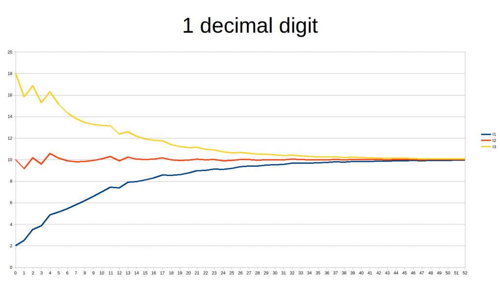
Let’s at least store a decimal digit:

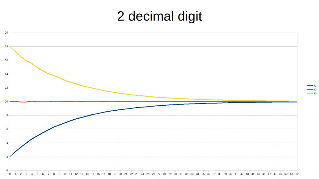
It is better, but still not so great. Let’s try one more digit:

This is definitely better and quite acceptable.

Number of decimal digits

It is thus advisable to use floating point numbers with sufficient digits to compute the UD otherwise we may experience some “clipping effects” such as these. This effect diminishes as we advance towards greater numbers, but then the question of the possible range for our integers arises. If we have selected 16 bits to store integer values, the bad news is that, even if starting with very small values as above and with a population of only 3 individuals, the total money mass reaches 67.410 after 86 years, which will make it impossible to continue storing transactions at that time. Of course, a currency for only 3 people is pretty useless. We should consider for instance 3000 people instead which is a more likely and yet still timid scenario. Even then, we reach the same threshold after only 1 year and a month, and the more participants the quicker the limit is reached.

Moving the floating point

At some point, it is necessary to use a mechanism to move the floating point over time. Indeed, as time goes by, it becomes impossible to store exponentially growing values. Of course, we could grow the number of storage bits over time as well, which would be a rather bad idea! Instead, it is much more simple to move the decimal point which changes the base for counting in steps of 10x. We only need to store the current “base” to know in which base a specific number is expressed into.

Distributing the UD over time

So far, we have considered that the UD is created every year. But it is actually best to create is as often as possible, to smoothen the inequalities over time. If we distribute the UD every year on Jan 1st, it is clear that if someone enters the economic zone on Dec 31st, he has an advantage compared to someone who enters on Jan 2nd.

Theoretically, the UD would be created (or distributed) over time continuously at every millisecond, actually every nanosecond or femtosecond. Unfortunately, that is practically impossible as computers are machines that don’t operate continuously and require more energy to perform more calculations. We need to find a compromise between computer calculations vs generated inequalities. It could be created every hour, every day or even every week, whatever seems “acceptable” to the community using the currency.

This has some effects on the currency itself as every UD generation causes the number of monetary units to grow which causes a gap in the value of each unit (more units mean less value for one unit).

Updating the UD over time

Another reason for the clipping may also be that the UD will not be revised every microsecond, and not even every time the UD is distributed, as it is a costly operation. Currently in the Ğ1 currency it is only revised every 6 months while it is distributed every day.

Firstly, if there aren’t enough significant digits, then we might have a clipping effect every 6 months or more due to the revision of the UD, which is quite bad. Then, every time the UD is revised, it causes a “jump” in the relative scale of prices.

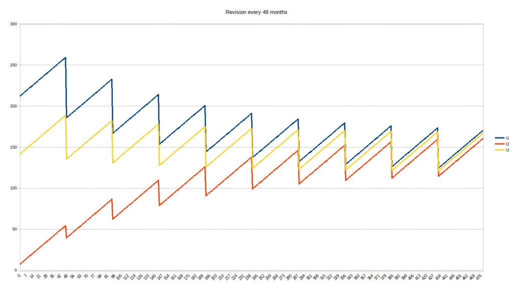
Let’s have a look at what happens if we revise the UD every 2 years instead of 6 months over a period of 40 years:

Have you noticed how the sawtooth effect is felt much more by the ones who own more money than the ones who own less? By the way, they don’t exactly experience minor changes on their accounts: the values suddenly drop by almost one third (exactly 28% in this case). This means that if people were to adjust prices, salaries and everything on the new DU, all prices would drop by 28% which is not acceptable for something that has only a purely technical cause that can be fixed.

To fix this further, we can revise the UD every 6 months:

Obviously, the sawtooth effect is still there, but on a much limited scale (4%) which seems proportionally more acceptable. However, we could probably consider revising the UD more frequently to avoid such a sawtooth effect.

Next is Part 3.

My Galileo Module – Part 1

There is a lot of material available in French on the original Galileo Module, which I already translated into English. But because I believe it is important to spread the information to other places than French-speaking communities, I am releasing my own version of the Galileo Module in English. This version will also explain to the reader the basics of the Relative Theory of Money so that no prerequisite is needed to read this blog article. This first part addresses the first part of the Galileo Module about changing frames of reference in a libre currency.

What is a libre currency?

A libre currency as defined by M. Laborde in his Relative Theory of Money (which I will shorten to “RTM”) is a currency in which all individuals in an economic zone create money equally and at regular intervals.  The amount of money created by all individuals is always a fraction of the existing money mass and every single individual at a given time creates exactly the same amount of money as the others. Thus, money is no more created by central entities, or banks, but rather by every living human, in full symmetry with his peers at a given time but also across generations. This is perfectly possible today thanks to blockchain technology. It is no coincidence in my opinion that the RTM was published in 2010, after the 2000 and 2008 crises but first and foremost shortly after the invention of the concept of blockchain in 2008.

(a) Changing Frames of Reference in Space

The spreadsheet for this part can be downloaded here.

Libre currency

We need to build a spreadsheet for the amount of libre money created by 3 individuals, I1, I2, and I3.

As explained above, libre currency functions as follows: regularly, every individual in the economic zone creates a share of money. This share of money is called a “Universal Dividend”. So at every interval, we need to calculate the total amount of money in circulation and multiply it by a celerity factor called c which is the percentage of the Universal Dividend. The result must then be divided it by the number of participants to get the Universal Dividend per person.

Note that the interval can be chosen randomly, but the shorter the better. In the current libre currency Ğ1 it is every day, but in this publication, we’ll stick to every year otherwise the spreadsheets could be quite huge!

The Absolute Reference Frame (counting monetary units)

Here is the beginning with 3 individuals I1, I2, and I3 who start in life with very different values in their accounts:

Year
I1 I2 I3 N Total Total/N UD c
0 0 10 100 3 110 36.67 3.67 0.1
  • N is the number of individuals
  • Total is the total amount of money available also called Money Mass, here it is simply the sum of the money of I1, I2, and I3
  • Total/N is the average amount of money available per individual
  • UD is the Universal Dividend per individual, which is Total / N ×  c
  • c is the celerity of the monetary creation, the percentage at which new money is created, here it is 10%=0.1. This means that the money mass will grow by 10% every year. Note that c cannot be chosen completely at random since it depends on the life expectancy of the population. 10% is an acceptable value for a population whose life expectancy is roughly between 35 and 80 years. For a population with an average 80 years life expectancy, the RTM predicts that values for c should be chosen between 6 and 10%.

At year 1, every single individual will create exactly one UD:

Year I1 I2 I3 N Total Total/N UD c
0 0 10 100 3 110 36.67 3.67 0.1
1 3.67 13.67 103.67 3 121 40.33 4.03  

We note right away that I1 has gone from 0 to 3+ units, while I2 sees a 30% increase of his money and I3 sees only a 3% increase in his money. The money mass is also growing which means that the UD for the next year is growing as well.

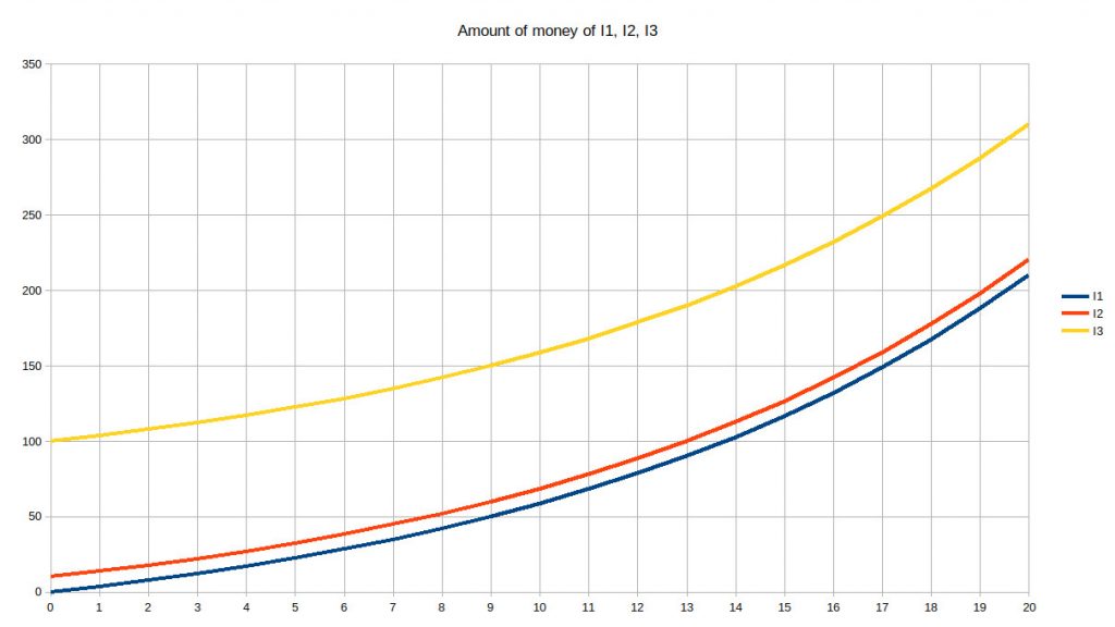
Because we are not computers I will stop showing the spreadsheet and show graphs instead which are much easier to read. Here is the graph of the amount of money over the first 20 years:

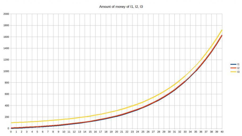
Unsurprisingly, this is an exponential curve. We can see that, over time, I1 who was the poorest, as well as I2 who was relatively poor compared to I3, are “catching up” with the richest – who still remains the richest. Now let’s extend this to 40 years, which is currently a half-life of a Westerner:

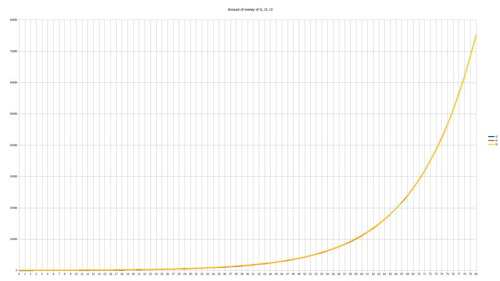
This time, it gets more difficult to see the difference between I1 and I2, and they are definitely catching up with I3. Let’s extend that to a full 80 years of life:

This time, the three curves are impossible to distinguish.

At first sight, this graph can be quite scary when we speak about money, especially about the total money mass. This reminds us of the Zimbabwe Dollar where an exponentially growing money mass is accompanied by exponential inflation, which is never a good thing when a state starts printing money like a crazy gambler:

The Relative Reference Frame (counting in proportion of the money mass)

Instead of counting monetary units, let’s change the frame of reference and use the percentage of the money mass as a reference.

Let’s go back to the first year of our 3 individuals and count how many percents of the existing money they possess:

  Year
I1 I2 I3
Absolute 0 0 10 100
Percentage   0 % 9.09 % 90.9 %

I1 has 0%, I2 has 9% and I3 has 91% of the total monetary units.

We have seen that in year 1 the amount of money they have has changed quite a bit:

  Year I1 I2 I3
Absolute 1 3.67 13.67 103.67
Percentage   3.03 % 11.29 % 85.67 %

Now instead of representing the charts with the monetary units, let’s draw the chart for the percentage of money they own over time and during 80 years:

It is now very clear that I1 and I2 are getting a higher percentage of the money over time, at the expense of I3. All accounts are mathematically drawn towards the mean of all accounts.

We can already note that they approximately reach the mean after 40 years. This is because we have chosen the celerity to be 10%. Let’s see what happens when we choose 6% instead of 10%, as those are the bounds specified by the RTM for a life expectancy of 80 years:

This time, the mean is roughly reached only after 80 years, which is totally in sync with the predictions of the RTM: the highest recommended values of c cause accounts to converge within a half-life, while lower values of c cause accounts to converge within a full life.

We will now stick with the value of c = 10% in the rest of the article.

Both the graph in relative value and absolute value can be translated into references where the sum of all money is 0 at all times. In other words, at every moment, we check the difference between every account with the average total money per individual instead of the actual amount.

In this reference frame, the quantitative graph is quite surprising as it basically doesn’t move at all. Indeed, the absolute monetary difference between the individuals doesn’t change. It is proportionally very different when you consider the total money mass, but in absolute values, it never varies since we consider that our individuals give exactly as much as they receive (either because they don’t make exchanges at all, either because their exchanges are perfectly balanced):

On the other hand, the relative frame does show the shrinking differences between the three since it takes into account the percentage of money that each of them possesses:

Note that in this frame of reference, we have suddenly lost all thought of “hyperinflation” that could have worried us in the absolute frame of reference. After all, this is a very stable way of creating money!

Taxation

Now that we’ve studied what happens with a libre currency, let’s check what happens when we apply a fully proportional tax, eg. we take a fixed rate of tax on the accounts, calculated that way for an account R(t):

tax(t) = c × (R(t) + 1) / (1 + c)

The total collected tax is then redistributed equally among every single individual.

Let’s calculate the tax for the first year:

Year I1 I2 I3 Total T1 T2 T3 Total Tax c
0 0 10 100 110 0.09 1 9.18 10.27 0.1

We can right away note that the tax on the rich is higher than the tax on the poor, which is normal since it is proportional. But we also note that there is an anomaly during the first year because the poorest has 0 and cannot be taxed. So we’ll adjust this special case to be 0 (is that fair – should he pay a tax to cover for this later?…). Now let’s see how it evolves over the next few years:

Year I1 I2 I3 Total T1 T2 T3 Total Tax
c
0 0 10 100 110 0 1 9.18 10.18 0.1
1 3.39 12.39 94.21 110 0.40 1.22 8.66 10.27  
2 6.42 14.60 88.98 110 0.67 1.42 8.18 10.27  
3 9.17 16.61 84.22 110 0.92 1.60 7.75 10.27  

We see that we take the same amount of taxes every year (10.27) except the first year because of the anomaly of I1. Globally, the trend seems to be the same as in libre money: all accounts seem to tend toward one another. Here is the chart when counting monetary units:

As predicted, the accounts all converge towards the average. But note that this is the graph in absolute values now, whereas in libre money the quantity of money was growing exponentially. Now let’s have a look at the graph in relative values:

Unsurprisingly, it does look the same, the only change being the scale.

So the big surprise (or not!) here is that libre currency is equivalent to a certain form of tax redistribution. The pleasant surprise with tax redistribution is that we don’t need to “burden” ourselves with the relative reference frame since the quantitative reference frame with tax redistribution is already behaving the same way as the libre currency.

Let’s proceed and collect taxes for our perfect redistribution system and put the RTM in the trash can! (humor – read on!)

Thoughts on taxation systems

Let’s have a look at tax collecting systems and their efficiency in the history of mankind.

If you dig just a little, you’ll find that tax evasion today is absolutely everywhere. It is said to leak more than 1,500 billion (yes, 1,500,000,000…) dollars every year in Europe alone. Besides, there is “illegal” tax evasion, but there is also “legal” tax avoidance which, thanks to the very lenient tax laws in many countries, allow the richest to avoid paying much taxes. The funniest part is that the French government is definitely not looking at big tax evaders, but looking instead at petty and insignificant tax evaders. They are really not seeing the elephant in the room!

This is actually not new. Tax evasion has been around for a while, actually at least since late Antiquity (2 different links).

In Ancient Greece, they actually found an original way of fighting tax evasion. Should we, too, incentivize our richest citizens to pay taxes in order to be revered and adored as benevolent philanthropists? Well, they already found the trick around that so it seems to be quite useless nowadays.

Let’s ask a simple question: why has tax evasion been always so popular?  It is easy to explain: human nature is such that we hate to lose something, which is the case with taxes. On the other hand, creating money is always winning something so it is much easier to accept, even if you are actually losing in proportion!

Oh well. Let’s dig back the RTM from the trash can and read it one more time. 😀

Libre currency vs tax redistribution first and last round

The huge advantage of a libre currency compared to a tax-collecting system is that there is no avoiding taxes and their redistribution, which is then simply carried out mathematically through monetary creation. Ingenious!

Part 2 is a little bit technical so if you’re not into technicalities about computers, you should skip directly to Part 3.

The Relative Theory of Money – Translation of the Galileo Module

“The Relative Theory of Money” is a book published in 2010 by a French engineer, Stéphane Laborde, who presents some very interesting thoughts and facts about money. He shows that, if we’re not careful enough, money creation can be the source of great inequalities. His book is a very good read for anyone, not only for those who wonder about money.

Within the book, many interesting questions are asked and answered. One of them is the “relativity of values”. To further study what is already analyzed in the book, the author offers a few “modules” in the form of exercises that can be done by anyone who wants to analyze further. Here is the translation in English of the first of these modules, the Galileo Module, the original (in French) can be found here: https://rml.creationmonetaire.info/modules/index.html

To be frank, at first sight it might look strange/gibberish if you’re not familiar with the RTM. I am publishing my own results of the module in English so that you can better understand what all this is about.

The Galileo Module

Theoretical data studies must be done from scratch. Economic data can be retrieved from various sources, or retrieved after verification of compliance from other contributors that have published their complete report of the module (which is the necessary condition to move to the next module). There are partial data known to date on the Duniter forum.

(a) Changing Frames of Reference in Space

  • create a spreadsheet representing a libre currency in the quantitative frame of reference with 3 individuals I1, I2, I3 over 80 years,
  • calculate the relative frame of reference,
  • create the two corresponding zero sum frames of reference,
  • create a separate sheet with the reverse relative / quantitative frames based on a tax which is redistributed using: individual tax(t) = c*(R(t)+1)/(1+c) collected and R(t+1) = R(t) + (collected tax(t) / 3) – individual tax(t)
  • perform a numerical analysis as well as a comparison of the graphs.

A Universal Dividend is equivalent to tax redistribution. Create a sheet and a graph to compare the two.

Note that there is a theorem that proves this by changing the frame of reference.

Quickly compare the discrete and continuous situations.

Think about Occham’s Razor.

(b) Simulate exchanges between I1 and I3

  • simulate some monetary exchanges in the spreadsheet in quantitative and relative frames,
  • discuss and reflect on the limited life expectancy of the actors.

(c) Changing frames of reference in time: replacement of generations

  • create a quantitative spreadsheet with [I1-I10] whose ages are from 0 to 72 years = 9 x 8 years
  • add [I11-I20] who are newcomers at regular intervals,
  • simulate replacing each of [I1-I10] over time with [I11-I20] in 80 years,
  • extend to 160 years, replacing each I10+k by I20+k,
  • create the relative frame and show it on a graph,
  • create the two corresponding zero sum frames of reference,
  • discuss the graphs on 160 years.

(d) Data to be downloaded to a spreadsheet

(e) Establish long term relative variations of different values

  • in euros,
  • in JSA/Welfare,
  • relative to the money mass (or better, 10% of the money mass),
  • relative to another economic value.

(f) General comments on the relativity of values

(g) Conclude

The next module is the Yolland Bresson Module.